Busy Excel spreadsheets can—frustratingly—grind to a halt, especially as you use the many functions and formatting options. The last thing you want is your worksheet to pause while executing a simple calculation, so check out these tips to keep your Excel spreadsheet running smoothly.
We recommend using the 64-bit version of Excel (which is installed automatically unless you manually select the 32-bit version), as it works better with large data sets, add-ins, and many other modern-day Excel features.
1. Don’t Over-Format Your Sheet
While you might think that adding formatting can spruce up your Excel worksheet, not only can it make your spreadsheet more difficult to read, but it can also slow it down. Any time you add formatting, whether that be using a fancy font, various font sizes, a range of colors, or different borders, you’re adding to the volume of the file. There are a couple of ways around this.
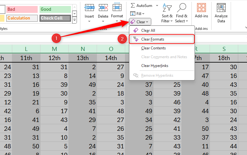
If you look at your spreadsheet and see that it does have lots of formatting, and you want to start afresh, press Ctrl+A to select all cells. Then, in the Home tab on the ribbon, head to the Editing group and click the “Clear” drop-down option. From there, click “Clear Formats.”
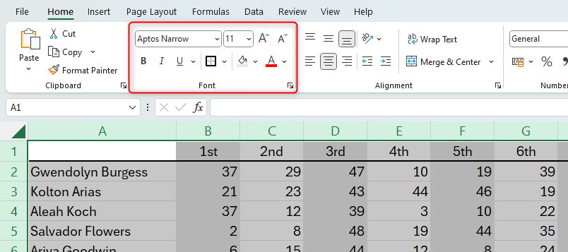
Alternatively, if you would prefer to keep certain formatting but remove other elements, after pressing Ctrl+A, work through the Font group in the Home tab to choose which formatting you want to remove.
Finally, you might have hidden formatting in the form of conditional formatting. Reducing the use of conditional formatting in your spreadsheet by managing the conditional formatting rules will help you to reduce the slugishness of your file.
2. Compress (and Limit) Your Images
High-resolution and large images and graphics within your spreadsheet will massively increase your file size. The best way to avoid this is to reduce the number of images and graphics in your workbook altogether, but if they are essential, use Excel’s in-built compression tool.
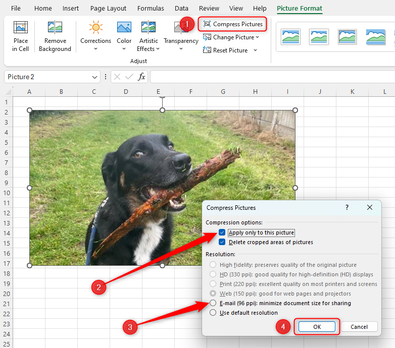
Select any image within your workbook and, in the Picture Format tab on the ribbon, click “Compress Pictures.” In the resultant dialog box, you can check the “Apply Only To This Picture” box if you only want to compress this image, or uncheck it if you want to apply the settings to all images in the file. Then, choose the best resolution that will work for you. If you have lots of images, choose the lowest resolution (96 pixels per inch). Finally, click “OK.”
3. Simplify Your Formulas
It’s inevitable that you’ll have formulas within your Excel workbook—after all, one of Excel’s biggest strengths is being able to perform dynamic calculations. However, complex formulas with lots of cell references and nested functions can be a huge contributor to a sluggish worksheet.
There are several ways to simplify your formulas. The first is to use named ranges within your formulas. Instead of referencing individual cells or ranges of cells within your formulas, referencing a named range means that Excel can more quickly identify and scan the specified data without having to work through a complex formula with lots of different cell references. What’s more, as well as speeding up your worksheet’s processing time, using named ranges makes your formulas easier to write, review, amend, and duplicate. The first step is to assign a name to a range of cells, and then use this name within your formula. For example, if we had a set of data in cells A1, B3, C5, D2, E9, F3, and G4, and we wanted to use these numbers to calculate an average, rather than typing
=AVERAGE(A1,B3,C5,D2,E9,F3,G4)
if we were to create a name—such as Results—to these cells, the formula would instead read
=AVERAGE(results)
Another way to simplify your formulas is to break down complex calculations into smaller ones. For example, if you wanted to work out the annual profit made by several employees for the past five years, rather than involving dozens of cell references, you could break down their profits per quarter, and then create an overall sum at the end of your row or bottom of your column.
Not only does this reduce the complexity of your formulas, but it also makes for easier analysis of your numbers.
Finally, instead of using complicated, nested IF formulas, you could use alternative functions. Depending on what you want to calculate, you could try using the VLOOKUP, CHOOSE, or LET functions, which require fewer arguments.
4. Avoid Blank Rows and Columns
Instead of having blank rows and columns to separate your data, use borders and colors. Having blank rows and columns increases your workbook’s file size and can delay Excel’s calculation processes. This will not significantly impact smaller workbooks, but having many blank rows and columns in between larger sets of data will. Along with the other tips in this article, removing blank rows and columns will definitely help to tidy up your Excel workbook and improve its performance.
5. Limit Changing Values
Certain functions in Excel change the value they produce any time Excel recalculates in your spreadsheet. For example, the =RAND function produces a new random number each time you make any changes to your worksheet, and =TODAY will update the cell value to reflect the current date. These are called volatile functions.
Because Excel has to continually work to update the values in the cells where you have volatile functions, it may cause a lag in your worksheet’s response time, and the more volatile functions you have, the lengthier the lag.
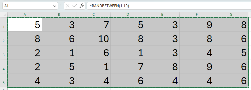
Other examples of volatile functions include =NOW, =RANDBETWEEN, =RANDARRAY, =OFFSET, and =INDIRECT.
The obvious way to limit the processing impact of volatile functions is to reduce their use altogether. For example, if you want Excel to produce a random list of numbers using =RANDBETWEEN, once the calculation has been made by Excel, consider making these values permanent. To do this, highlight all the numbers created by the calculation and press Ctrl+C.
Then, select the top-left cell of the random array. In the Home tab on the ribbon, click the paste drop-down arrow, and choose the “Values” icon.
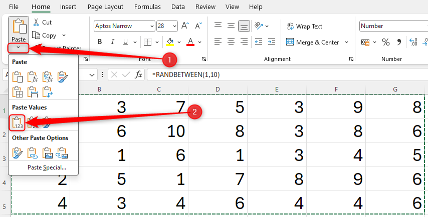
You will see that the numbers change within your parameters one more time (as they were still volatile right up to the point when you pasted their values), but they are now in your spreadsheet as true numbers and will not change when Excel recalculates.
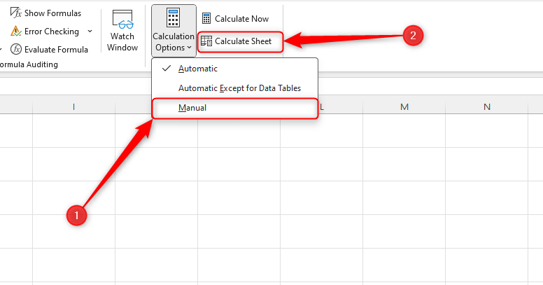
Another way to prevent volatile functions from slowing down your spreadsheet is to turn off automatic calculations. In the Calculation group of the Formulas tab on the ribbon, click “Calculation Options” and check “Manual” to tell Excel not to update volatile functions automatically. Then, when you’re ready for your volatile functions to update, click “Calculate Sheet.”
This means that they will only potentially slow down your spreadsheet when you’re prepared for this to happen, rather than with every change you make.
6. Clear Up Named Items
As we mentioned in tip 3, using named ranges can help you to simplify your formulas and generally tidy up your workbook, but it’s important to make sure you don’t have redundant names or multiple names for the same array of data. Doing so will add an extra layer of processing that Excel has to address when you’re opening up, working in, and closing your workbook.
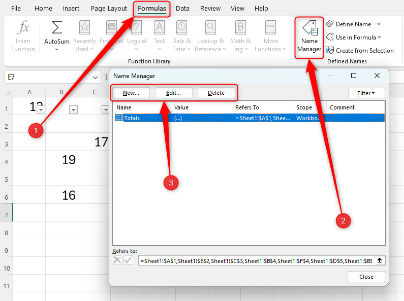
To clear up all the named items in your workbook, in the Formulas tab on the ribbon, click “Name Manager.” When the dialog box opens, you’ll see all the named ranges in your workbook. Review these manually, clicking “Delete” to remove any unused named ranges and clicking “Edit” to tidy up their names.
7. Check Performance
If you have exhausted all the tips above and find that your workbook is still under-performing, you can force Excel to run through a check-up on your file. Originally introduced to Excel for the web in 2022 and extended to the Windows Excel app in 2024, Excel’s Check Performance tool looks for excess formatting, unneeded metadata, unused styles, and other issues that might affect the speed of your workbook.
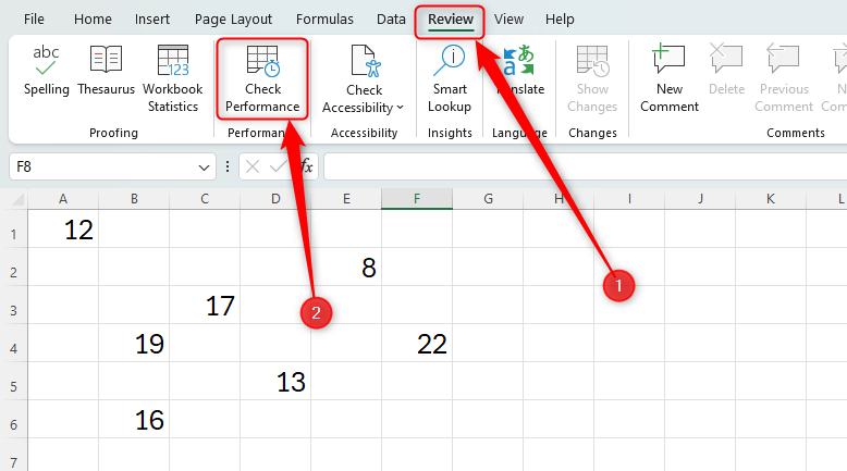
In the Review tab on the ribbon, head to the Performance group and click “Check Performance.”
A sidebar will then open on the right-hand side of your window containing guidance about what you can do to improve your workbook’s performance.
If you’ve run through these tips and find that Excel is still working slowly, maybe the cause of the issue is not the Microsoft 365 app—you may need to increase your overall PC performance instead.