The Low-Volatility Factor And Occam’s Razor

The low-volatility premium may be the most compelling anomaly in financial markets: Less risky securities outperform their riskier counterparts over the long term.

Empirical tests of the capital asset pricing model (CAPM) first documented this counterintuitive phenomenon more than a half-century ago. It emerged not in a search for alpha but rather as an unwelcome reality, an unintended consequence of theory testing, and remains poorly understood to this day.

This makes the defensive low-volatility factor unique and sets it apart from other factors.

Since the low volatility factor defies a risk-based explanation, academics who believe in efficient markets have trouble accepting it. Indeed, Eugene Fama and Kenneth French left low volatility out of their three-factor and five-factor models.

Practitioners, by contrast, often struggle to capitalize on the factor because of the high risk associated with it relative to its benchmarks and because of leverage constraints and potential career risks.

Such complexities and hurdles make low volatility a special animal within the expanding “factor zoo.”

Yet, the low-volatility factor is both resilient and robust.

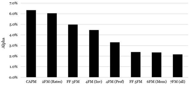
Here, by applying the principle that the simplest explanation is usually the most accurate – Occam’s razor – we make the case for low volatility. The graphic below shows how low volatility interacts with other factors. Even after seven cuts or slices, the factor still performs. If it keeps its alpha after so many slices, its simplicity must be key to its significance.

The Starting Point: CAPM

Using US market data from July 1940 to December 2023, we measure the volatility factor much like a Fama and French style factor, by taking a long position on low-volatility stocks and a short one on their high-volatility counterparts. Over this period, the low volatility premium (VOL) equals 6.4% with a beta that by construction is very close to zero. The CAPM alpha is 6.3% per annum with a t-stat of 5.3, far above the critical levels Campbell Harvey recommended to minimize the risk of finding “fake factors.”

Low-Volatility Premium (VOL) Controlled for Other Factors, July 1940 to December 2023

The First Slice, 2FM (Rates): Two Factors, Equities and Bonds

When the CAPM was unveiled, Richard Roll’s critique was that bonds and other assets should be included in the market portfolio. Since low-volatility stocks resemble bond-like stocks, this higher rate sensitivity could be an explanation. Still, a two-factor regression that includes both equities and bonds lowers VOL’s alpha by only 0.3%.

Second Slice, FF 3FM: Fama-French Three-Factor Model

One explanation of the low-volatility factor is that value is often defensive. While the relationship is time-varying, on average volatility loads positively on value and negatively on size. The classic three-factor Fama-French regression, which includes both the value and size factors, reduces VOL’s alpha by 1.1%.

Third Slice, 4FM (Inv): Three-Factor Model Plus Investment

Fama and French augmented their three-factor model with two more factors – investment and profitability – in 2015. We find the investment factor accounts for about 0.5% of VOL’s alpha. This makes intuitive sense, since conservative, low-investment firms tend to exhibit less volatility.

Fourth Slice, 4FM (Prof): Three-Factor Model Plus Profitability

Of these two new factors, profitability has a much stronger relationship to volatility and accounts for 1.2% of VOL’s alpha. We find that unprofitable firms tend to be very volatile, even as their profitable peers do not always demonstrate the opposite. Thus, the short leg drives most of this result.

Fifth Slice, FF 5FM: Fama-French Five-Factor Model

Combined, these five factors bring VOL’s alpha down by 0.9%. This indicates that investment and profitability are different dimensions of the quality factor that interact with value and size.

Sixth Slice, 6FM (MoM): Five-Factor Model Plus Momentum

The most dynamic factor, momentum, generates high gross returns but requires considerable turnover, which erodes net returns. This is why Fama and French did not include it in their five-factor model. When we add momentum, the VOL premium does not rise or fall.

Seventh Slice, 7FM: The Kitchen Sink

In our final, all-inclusive “kitchen sink” regression, VOL’s alpha declines by 0.2% and is still standing at a statistically significant 2.1%.

All this demonstrates low volatility’s overall robustness. The factor’s outperformance survives critiques from all different angles. By applying Occam’s razor to the factor zoo and slicing low volatility every which way, the strategy still stands out as the premier factor. If it takes five or six factors to explain it, low volatility may not be that bad after all.

To take it one step further, by integrating value, quality, and momentum into a “Conservative Formula,” we create an enhanced low-volatility strategy that beats VOL along with all the other factors. The following figure shows how the Conservative Minus Speculative (CMS) portfolio fares after each of our previous cuts. The alpha starts at 13.3% and only falls to 8.2% after all seven slices.

Enhanced Volatility Premium (CMS) Controlled for Other Factors, July 1940 to December 2023

Amid low demand for defensive investing during the recent tech-driven market rally, the case for low-volatility investing may be stronger than ever. In a market that often overlooks it and a world where the obvious is often overcrowded and overvalued, the low-volatility anomaly stands as a testament to the power of contrarian thinking.

Sometimes, the less-trodden path offers the better journey. As we look ahead, the question remains: Will the market eventually catch up to this hidden gem, or will low volatility continue to be the market’s best-kept secret?

Disclaimer: Please note that the content of this site should not be construed as investment advice, nor do the opinions expressed necessarily reflect the views of CFA Institute.

Original Post

Editor’s Note: The summary bullets for this article were chosen by Seeking Alpha editors.