It’s all well and good having a complicated Excel spreadsheet full of data and formulas, but if it’s not presented neatly, it can cause more problems than it solves. We’ll show you six tips that you can use to tidy up your spreadsheet and communicate your data more clearly.
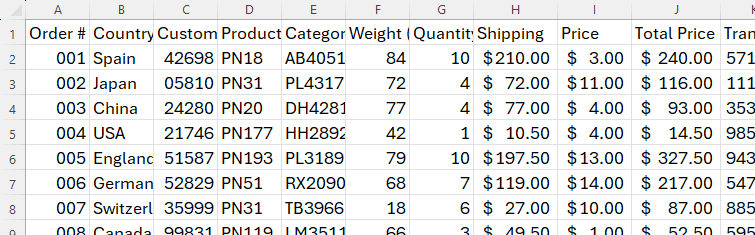
This unformatted spreadsheet has several readability issues which we’ll address throughout this article.
Tip 1: Freeze Your Rows and Columns
Our spreadsheet is very large with lots of rows and columns, which means that when we scroll down or across, we can’t see the row or column headers. Freezing your column and row headers will keep them permanently in view, no matter where you are on your sheet. To see your freezing options, open the “View” tab on the ribbon, and click “Freeze Panes” in the Window group.
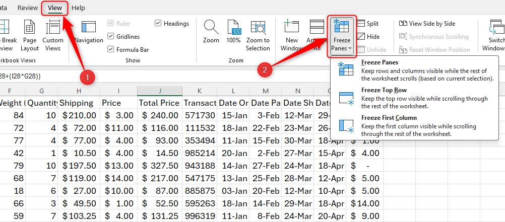
Freeze Top Row and Freeze First Column: As their names suggest, these two options let you freeze row 1 or column A. Excel chooses these as quick-access freezing options because this is usually where your row and column headers sit. Note, however, that these options do not allow you to perform both actions—if you click one of these two options and then click the other, only the last option you chose will be performed on your sheet.
Freeze Panes: If you want to freeze more than just one row or column (if, for example, you have more than one header row), or decide that you want to freeze columns and headers, this option is the one for you.
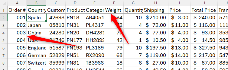
To freeze several rows at the top of your sheet, select the first row that you don’t want to freeze and click “Freeze Panes.” So, if you want to freeze rows 1 and 2, select row 3, and click “Freeze Panes.” Similarly, if you want to freeze columns A and B, select column C, and click “Freeze Panes.” To freeze rows and columns together, you need to click the highest and left-most cell that you don’t want to freeze, and click “Freeze Panes.” An example will make this clearer.
In our example below, we want to freeze row 1 and column A, so we will freeze panes from cell B2. Excel will then draw a thicker line to demonstrate where the freezing has taken effect.
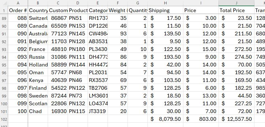
Now, when you scroll down or across, you’ll see that the headers remain viewable.
To unfreeze the panes, go back to the “View” tab on the ribbon, click the “Freeze Panes” button, and choose “Unfreeze Panes.” Pressing Ctrl+Z (undo) will not work.
Tip 2: Don’t Overuse Cell Borders
It’s often tempting to add borders to your cells to make things clearer, but this can make your spreadsheet look clunky and unprofessional. After all, Excel already has its in-built gridlines to help you differentiate between cells. Instead, color your cells or use horizontal borders only.
In this example, we have added a totals row at the bottom of our spreadsheet, and we want to clearly distinguish this from the main data in our table.
First, select the row you want to affect (in our case, row 102). Then, open the “Home” tab on the ribbon, and use the border and color options to format this row.
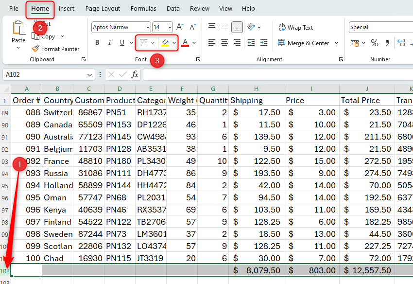
We recommend you apply a top border only, and use a light color fill, such as light blue or gray.
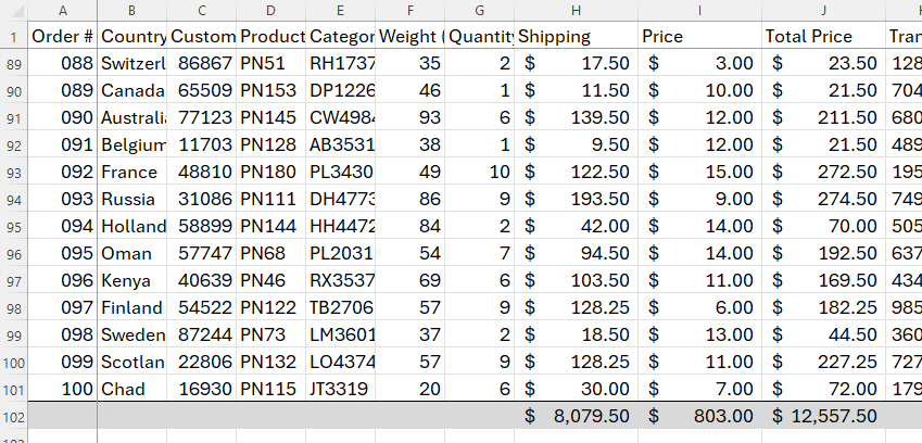
For more border or color options, right-click the row number, and click “Format Cells.” Whichever color you choose, use variants of that same color throughout your spreadsheet (tip 3). Furthermore, you can let Excel create the table formatting for you (tip 5).
Tip 3: Use Consistent Formatting
We’re making good progress with our spreadsheet, but one thing that still stands out is that we can’t see the column headers fully as the text won’t fit into our cell width. Follow two steps to achieve this consistently.
First, if you have lengthy column headers, wrap the text in the cell. This means that the text runs onto the next line to fit into the chosen cell width. To do this, highlight the header row, and open the “Home” tab. Then, in the Alignment group, click “Wrap Text.”
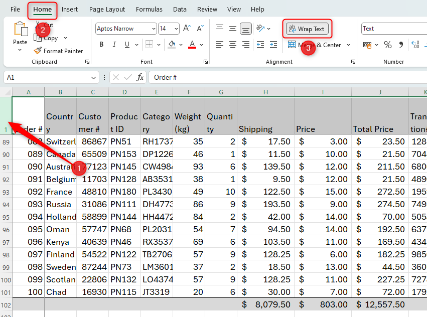
You will see that the text in each cell along this row has now adjusted to fit the cell width.
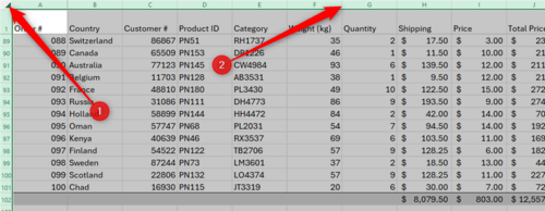
However, as some of the words are longer than the cell width, they are split into two lines. So, the second step is to adjust the column widths. You can adjust column widths individually, but we want them to be the same, so that there’s an aesthetic consistency across our sheet.
To do this, highlight all cells in the worksheet by clicking the top-left cell reference square. Then, adjust one of the column widths by clicking and dragging between two column headers (you’ll see your cursor change to a two-way arrow), and they will all widen together. Glance at your table to make sure you’re happy that the text and data fit nicely. If you’re not, simply adjust them again until they look great.
Once you’ve achieved a suitable cell width, click anywhere on your sheet to deselect the cells. You’ll notice that doing this makes your spreadsheet far less cramped, which, again, is pleasing on the eye.
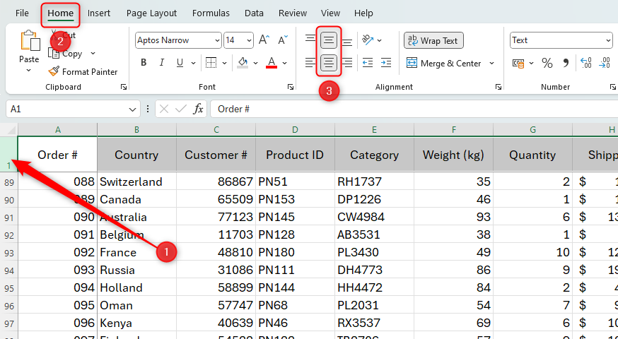
We’d also recommend that you center-align your headers vertically and horizontally to add that extra professional quality. Select the header row and click both center alignment icons in the Alignment group on the Home tab.
In Excel, by default, text aligns to the left and numbers align to the right. You may wish to make these all the same—or even center-align all your data—to increase the readability of your data.
Also note the following tips to achieve consistent formatting:
- Use the same font and font size throughout your workbook, choosing a typeface that is easy to read, such as Arial, Calibri, or Aptos. If you need to emphasize something, either use bold font or color the cell background.
- Choose a color palette. When choosing cell or font colors, follow the vertical columns in the theme colors to use different shades of the same colors. Not only does this make your spreadsheet more professional, but it also means that if you use conditional formatting, you can choose a color that will stand out against your chosen color palette.
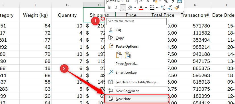
Tip 4: Use Notes to Avoid Too Much Text
Having too much text in a cell defeats the objective of having an easy-to-read Excel sheet. To get around this, right-click the relevant cell and click “New Note.” Then, rather than filling the cell with lots of text, you can add extra information to the note.
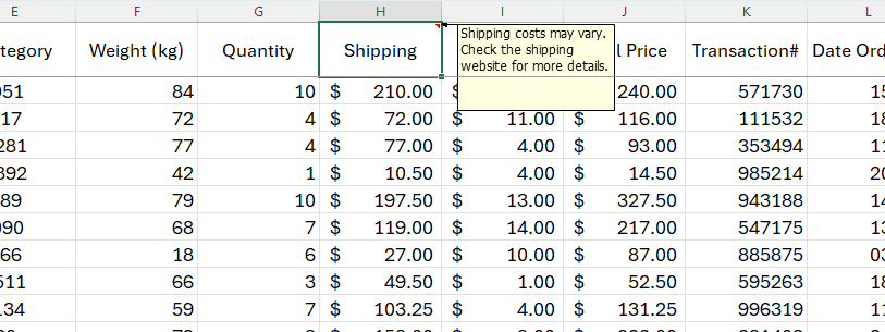
Type the details you want to add to this cell’s note, and then click away from the note to save and close it. You’ll then see that the cell has a small red marker in the corner to tell you there’s a note. Hover over any cells containing this red marker to see the note.
To edit or delete the note, simply right-click the cell again and click “Edit Note” or “Delete Note.”
Tip 5: Let Excel Create Your Charts and Tables
A quick and easy way to improve your Excel sheet’s appearance and display your data effectively is to use the in-built chart and table functions.
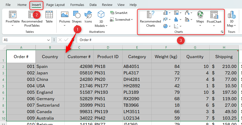
To create a chart from your data, highlight the relevant data, click “Insert” on the ribbon, and choose a chart that works well for you.
You can also tell Excel to format your tables. To do this, highlight all the data in your table, including the header row or column. Then, open the “Home” tab, and click “Format As Table” in the Stypes group, and choose a layout that works with your chosen color palette.
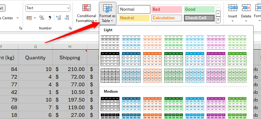
With any cell in your table selected, go to the “Table Design” tab and choose from the other options to amend your table styles.

Tip 6: Share as a PDF to Lock Your Layout
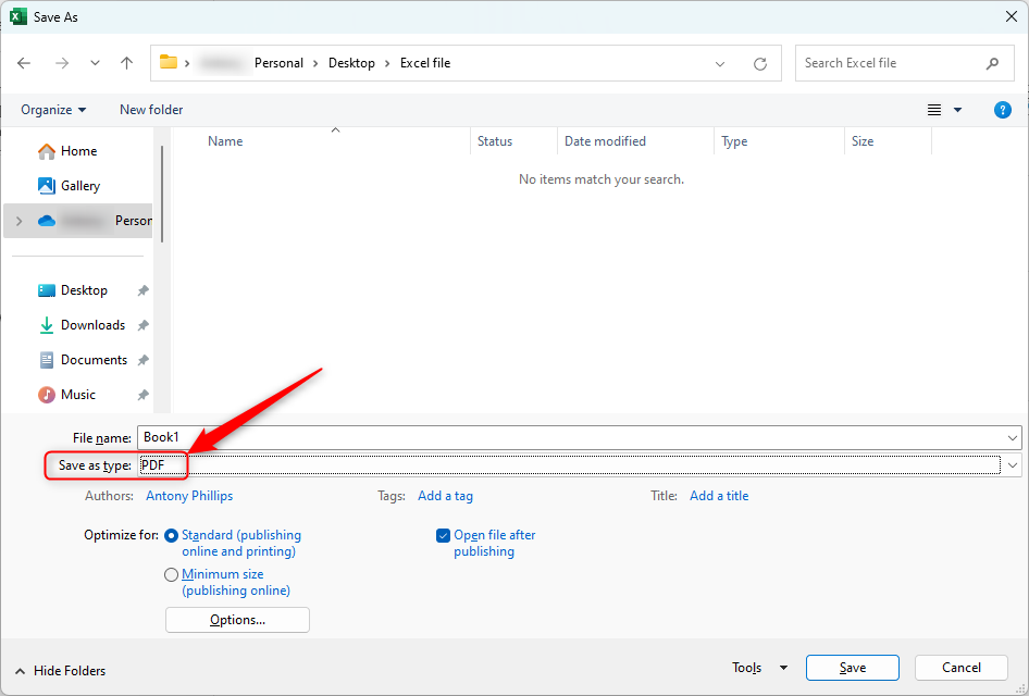
Now that you have a professionally formatted Excel sheet that is easy to read, it’s ready to share and print. Excel’s formatting can change if you share the workbook with someone who will open it on their mobile or a computer with an older version of Excel, and all your hard work might be undone. To keep your layout intact, save your worksheet as a PDF.
Click File > Save (or Save As) > Browse, and in the window that appears, change the Save As Type option to “PDF.”
If you know what type of spreadsheet you’re creating, whether that be a budget report or calendar, try using one of Excel’s templates, which are already set up and formatted to look slick and professional.