Excel has hundreds of functions that can help you to quickly and accurately perform calculations, among which are the AVERAGE functions. You might want to calculate the average sales figures, get the average of a group of data that contains numbers and text, or work out the average of all student scores over a certain number.
How Many Average Functions Are There in Excel?
There are four AVERAGE functions and each has different uses:
- AVERAGE: This produces the arithmetic mean (the sum of all numbers divided by the number of values) of a set of data, ignoring anything that isn’t a number.
- AVERAGEA: This returns the mean of a set of numbers, text, and logical arguments.
- AVERAGEIF: This calculates the arithmetic mean of a set of numerical data that fulfill a single criterion.
- AVERAGEIFS: This tells you the arithmetic mean of a set of numerical data that fulfill several criteria.
Let’s explore these in more detail.
How to Use AVERAGE in Excel
To calculate the average in Excel, use the following syntax:
=AVERAGE(A,B)
where A is the first number, cell reference, or range, and B is up to a maximum of 255 additional numbers, cell references, or ranges to include in the average calculation.
In this example, we have a set of seven students and want to calculate their average exam score.
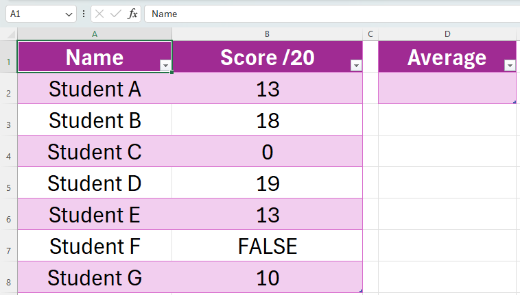
As you can see, Student C scored 0 and Student F has yet to take the exam. As a result, we want Excel to work out the scores of those who have taken the exam (all students except for Student F).
To do this, we would type the following formula into cell D2:
=AVERAGE(B2:B8)
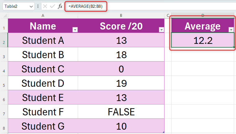
The AVERAGE function includes 0 within its calculations, but ignores all empty cells, text, and logical values (TRUE or FALSE). So, we can be confident that this calculation will include Student C’s score, but ignore Student F’s score.
If any of the values being used in the AVERAGE calculation were to contain one of Excel’s formula errors, the calculation would not work.
To save time, you can instead calculate the average through a few simple clicks. First, select your data to average, click the “Home” tab on the ribbon, and in the “Editing” group, click on the drop-down arrow next to the sigma (Σ) symbol. From there, click “Average”. The result will appear at the end of your data.
How to Use AVERAGEA in Excel
AVERAGEA works in a very similar way to AVERAGE, but includes more than just numbers within the calculation. Here’s the syntax for this function:
=AVERAGE(A,B)
where A is the first value (including numbers, logical values such as TRUE or FALSE, and text), and B is up to a maximum of 255 additional values to include in the average calculation.
The AVERAGEA function is useful if you have a mixed set of data containing numbers, logical values, and text, and you want to include them all within your calculation.
Taking the same set of data that we used in the example above, we now want to work out the average using AVERAGEA.
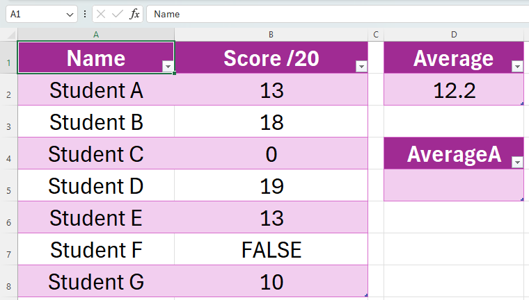
In cell D5, we would type the following formula:
=AVERAGEA(B2:B8)
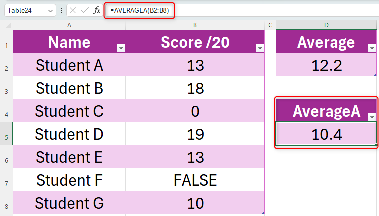
Unlike the AVERAGE function, which ignores logical values, the AVERAGEA calculation includes FALSE within the calculation as 0. If this were instead TRUE, this would be counted as 1. As a result, in our example, Student C’s score of 0 is included, and Student F is also calculated as having scored 0. This is why the result is lower for this calculation than the previous one.
AVERAGEA counts any other text as 0 (for example, if you type FOUR, this is still represented as 0, and not 4), and ignores empty cells.
As with AVERAGE, if any of the values being used in the AVERAGEA calculation were to contain one of Excel’s formula errors, the calculation would return an error.
How to Use AVERAGEIF in Excel
AVERAGEIF effectively performs two calculations in one go, first identifying data that meet a certain criterion before then finding the average of these data. AVERAGEIF uses the following syntax:
=AVERAGEIF(A,B,C)
where A is the range of values or cells to include in the average, B is the criterion, and C (optional) is the actual set of cells to average. Confusing? Let’s look at this example.
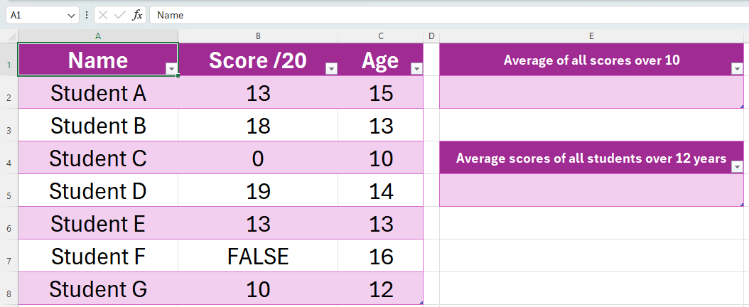
We want to work out two things from this table. First, we want to find the average score of all students who scored more than 10 in the exam, and second, we want to work out the average scores of all students over 12 years of age.
To work out the average score of all students who scored more than 10, we would use the following formula:
=AVERAGEIF(B2:B8,">10")
Notice two things in this formula. First, the criteria must always be enclosed in double quotes. Second, we’ve only included two arguments within the parentheses, as there’s no need to refer to any other data elsewhere within our calculation.
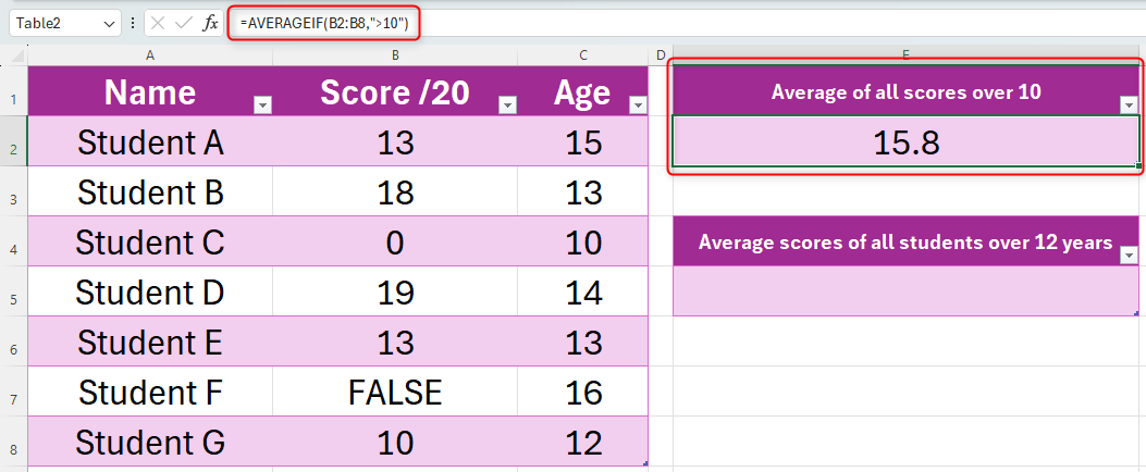
This has correctly picked up the scores of Students A, B, D, and E, as these are all more than 10.
To work out the average scores of all students over 12 years of age, we would use the following formula:
=AVERAGEIF(C2:C8,">12",B2:B8)
Notice the difference between the two formulas. Where the previous calculation contained two arguments, this one contains three, as we are assessing two sets of data.
The “C2:C8” part of the formula tells Excel to look in that range (the students’ ages) for the criteria, the “>12” part tells Excel to identify any values over 12 in the C2:C8 range (the students’ ages), and “B2:B8” (the students’ scores) is the part being averaged.
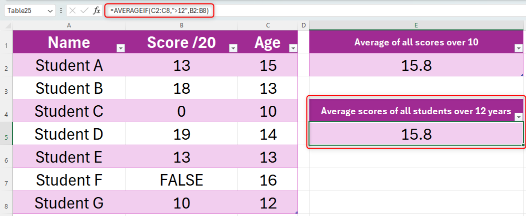
This has correctly picked up the scores of Students A, B, D, and E, as they are all over 12 years of age. The calculation also ignores logical values, which is why it hasn’t considered Student F, even though they are over 12 years old.
The criteria used in AVERAGEIF can use one of Excel’s six logical operators—these are > (greater than), < (less than), = (equal to), <= (less than or equal to), >= (greater than or equal to), or <> (not equal to)—and wildcards (* and ?). If you want to include an actual question mark or asterisk, add a tilde (~) before the character.
How to Use AVERAGEIFS in Excel
The AVERAGEIFs function allows you to include several criteria to assess before calculating the average. It works using the following syntax:
=AVERAGEIFS(A,B,C)
where A identifies the cells to average, B is the cells used to identify the criteria, and C is the criteria. There can be up to 127 criteria, so multiple pairs of cells (B) and criteria (C) can be used.
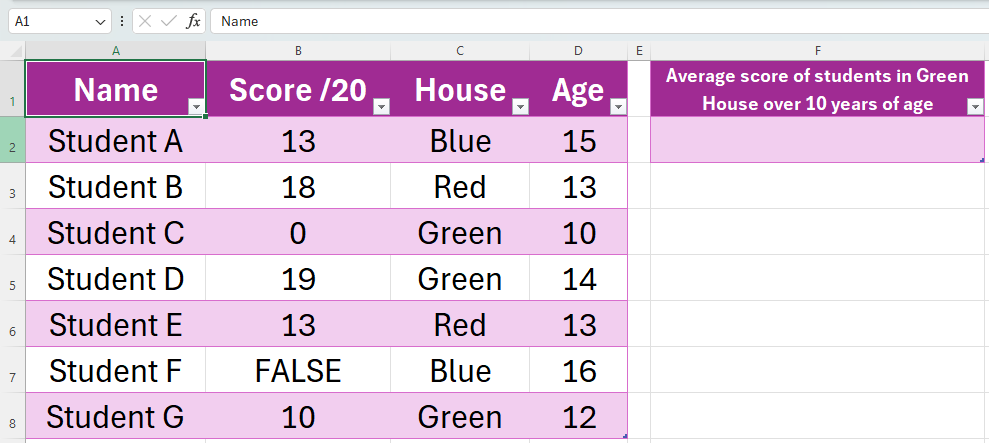
Take this example, where we want to work out the exam scores of students in Green House over the age of 10.
To do this, we would use the following formula:
=AVERAGEIFS(B2:B8,C2:C8,"Green",D2:D8,">10")
“B2:B8” contains the data to be averaged (the students’ scores), “C2:C8” is the first range to be tested with the criterion of “Green” (the student’s house), and “D2:D18” is the second range to be tested with the criterion of “>10” (the student’s age).
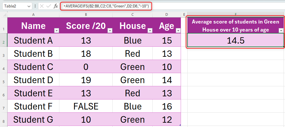
This has correctly averaged the scores of Students D and G, as they are both in Green House and are over 10 years old.
Other things to note about AVERAGEIFS:
- TRUE is counted as 1, and FALSE is counted as 0.
- In the criteria, you can use a question mark (?) as a wildcard to match any single character, or an asterisk (*) as a wildcard to match any sequence of characters. Use a tilde (~) before the character if you’re looking to identify an actual question mark or asterisk.
As well as using AVERAGEIF and AVERAGEIFS, you can sort and filter data in Excel to only show certain figures within your tables.