Goehring & Rozencwajg Q4 2023 Natural Resource Market Commentary

THE NORWEGIAN ILLUSION

“Electric vehicles (EVs) are piling up on lots across the country as the green revolution hits a speed bump, data show.” USA Today, November 14, 2023

“Hertz Global Holdings announced Thursday it planned to cut one-third of its global EV fleet over the year. Following the announcement, Hertz CEO Stephen Scherr suggested the road to electrification could be bumpier than anticipated.” Bloomberg, January 11, 2024

Starting mid-point last decade, the investment community became convinced EV adoption would quickly surge. EV penetrations would become so great that global oil consumption would imminently peak, or so consensus opinion widely believed. 2019 was repeatedly referenced as the year that oil demand would peak and then decline. In retrospect, these concerns were misplaced. Despite the massive COVID-19 disruption, oil demand in 2024 should reach 103 m b/d – 2.3 m b/d greater than 2019. Undeterred by the surprising surgein demand, many analysts remain convinced that “peak oil demand” is still imminent. The investment community’s belief that EVs will displace the internal combustion engine remains as strong as ever. We vigorously disagree.

In our last letter, we predicted that global energy demand would consistently exceed expectations for the next twenty years. Never before have so many people been simultaneously in their period of energy-intensive economic development. Our essay focused broadly on total energy demand and specifically avoided oil consumption. Our choice was deliberate: we wanted to highlight the critical drivers of total energy demand and avoid getting distracted by the debate on EV penetration. Today’s essay focuses on oil and explains why we believe demand will surprise to the upside for years to come.

Our research shows that EVs will struggle to achieve widespread adoption despite massive subsidies and the growing threat of outright internal combustion engine (‘ICE’) bans. After carefully studying the history of energy, we have yet to find an example where a new technology with inferior energy efficiency has replaced an existing, more efficient one. Despite claims to the contrary, our research suggests EVs are less energy efficient than internal combustion engine automobiles. As a result, they will fail to gain widespread adoption.

Our claim is controversial; most pundits insist EVs are far more efficient. We believe the ICE is clearly the winner once the energetic costs of both the battery and the renewable power required to make “carbon-free” EVs are considered.

Although governments can encourage EVs through either subsidies or ICE bans, these measures will likely fail, as consumers will ultimately refuse to embrace a new technology that sports inferior energy efficiency. Better examples couldn’t exist than Ford and Hertz dramatically scaling back their EV initiatives due to lower-than-expected consumer interest.

Mitigating carbon emissions is central to the case for electric vehicles. Advocates argue that displacing fossil fuels is essential to curbing global warming. We disagree. Replacing ICEs with EVs will materially increase carbon emissions and may worsen the problem. Manufacturing an electric vehicle consumes far more energy than an ICE. Most of this additional energy is spent mining the materials for and manufacturing an EV’s giant lithium-ion battery. Mining companies use energy-intensive trucks, crushers, and mills to extract each battery’s nickel, cobalt, lithium, and copper. The manufacturing process consumes vast amounts of energy as well. Many analysts eagerly tout the carbon savings from displaced fossil fuels without adequately accounting for the battery’s increased energy consumption. Once these adjustments are made, most, if not all, of the EV’s carbon advantage disappears.

If our models are correct, EVs will fail on two fronts: they are less energy efficient than the ICEs they are trying to replace and their adoption will do little to mitigate carbon emissions.

Policymakers often tout Norway as the ultimate EV success story. Thanks to massive subsidies, EVs made up 80% of all Norwegian new car sales in 2022 and currently account for 20% of the total car fleet. Policymakers hope all developed countries will ultimately adopt Norway’s model. However, upon closer inspection, Norway’s experience does more to warn of EVs’ shortcomings than advocate for their adoption.

The first problem is financial. The Norwegian government offers consumers massive subsidies to purchase an EV. New vehicles are exempt from several onerous taxes and the 25% VAT. On average, a large new ICE would be subject to $27,000 in various taxes; an equivalent EV would pay none. Next, Norway exempts EVs from any road or ferry tolls and allows them to use bus lanes, offers free parking and charging in municipal areas, and ensures “charging rights” in apartment buildings. Although Norway rolled back some of these operating subsidies starting in 2017, an Oslo resident can still expect these benefits to total $8,000 annually.

Norway is one of the wealthiest countries in the world, with a per capita GDP of $106,000 in 2022. Despite its impressive wealth, the government must still financially incentivize its citizens to purchase EVs.

The benefits are starting to take their toll on Norway’s finances. At nearly $4 billion annually, Norway spends as much on EV subsidies as on total highway and public infrastructure maintenance. The program has also raised significant issues around equality in Norway. EV subsidies favor high-income urban citizens, who take advantage of free tolls, parking, and charging and avoid the onerous tax on larger luxury vehicles. Several populist-leaning political groups in Norway have made so-called “elitist” EV subsidies a focal point of their platform.

Amid growing scrutiny, the government has actively sought to reduce several subsidies. Municipal parking is no longer free, and passengers (although not the vehicles themselves) are subject to certain tolls. The government also introduced a partial purchase tax on new EVs. Proponents have warned that any rollback of subsidies will surely harm EV penetration and offer Sweden as a case study, where, in 2022, the elimination of several subsidies precipitated a 20% drop in EV sales.

More important, EVs in Norway have not affected fossil fuel demand or carbon emissions as expected. Although oil demand and carbon emissions have fallen by 15% since 2010, most of this is unrelated to EV sales. Over the period, total oil demand fell by only 34,000 b/d, with gasoline and diesel making up a mere 10% of the decline. Most of the decline came from heating, lighting, and petrochemical demand, which we estimate collapsed by more than a third. Despite 20% of all vehicles on the road now being electric, Norway’s gasoline and diesel demand fell by a mere 4%.

Our data suggests that Norwegians are reluctant to give up their ICE vehicles, even after purchasing an EV. We calculate that two-thirds of Norway’s EV households own at least one ICE vehicle. From 2010 to 2022, Norway added 550,000 EVs, but the number of ICE vehicles on the road, rather than falling, increased by 32,630. While the population grew by 11%, the total number of passenger cars grew by 25%. When an EV household prefers to avoid a road or ferry toll, have access to free parking or charging, or avoid congestion by using bus lanes, they use their EV. When they visit their hytte in the mountains, they use their ICE. The impact has been so material that advocates have lobbied for a government-funded ICE scrappage program,another veiled EV subsidy.

Unsurprisingly, electricity demand has surged as Norway shifted from fossil fuels to electricity for transportation, heating, and lighting. Since 2010, Norwegian electricity demand rose an impressive 20%. Total primary demand for all forms of energy increased by 5%. The data suggests that a widespread shift to EVs did little to reduce overall energy consumption despite claims they are far more efficient.

The shift from fossil fuels to electricity has reduced Norway’s CO2 by an impressive 16%, an achievement lauded in the press. Far less discussed, however, is how the US lowered its emissions by 16% over the same period, by switching from coal to natural gas in its power generation.

Using Norway as a model for CO2 reduction would be a mistake. Far more than any other country in the world, Norway benefits from its vast hydrological potential which generates nearly 92% of all electricity carbon free. Therefore, a move from fossil fuels towards electricity will significantly impact Norway’s carbon emissions more than anywhere else on Earth.

Furthermore, Norway imports all domestic EVs. As we discussed, EV manufacturing is incredibly energy-intensive, mainly to build the battery. In Norway’s case, none of this additional energy is reflected in their domestic demand figures. China manufactures most lithium-ion batteries and 80% of all EVs. Coal accounts for 60% of their total energy supply.

We estimate an average EV consumes 60 MWh to manufacture, of which the battery represents half. Therefore, manufacturing Norway’s 579,000 EVs (all the EVs on the road today in Norway) requires 35 twh, equivalent to 25% of the total annual Norwegian electricity demand. Given that China emits 600 grams of CO2 per kwh (China is where almost all of Noway’s EV batteries are manufactured), we calculate Norway’s EV fleet would emit 21 mm tonnes of CO2. Norway’s gasoline and diesel consumption fell by a meager 3,200 barrels per day or 50 mm gallons per year. Assuming 9 kg of CO2 per gallon of gasoline or diesel, Norway’s entire EV fleet mitigates a mere 450,000 tonnes of CO2 per year, compared with an upfront emission of 21 mm tonnes. In other words, it would take forty-five years of CO2 savings from reduced gasoline and diesel consumption to offset the initial emissions from the manufacturing of the vehicles. Since an EV battery has a useful life of only ten to fifteen years, it is clear that Norway’s EV rollout has increased total lifecycle CO2 emissions dramatically. Incredibly, this is true despite Norway having the lowest carbon hydroelectricity in the world. Even if China were to reach its overly ambitious targets for wind, solar, and nuclear power by 2035, we calculate that the carbon “payback” would still exceed twenty years. Realistically, the only way for EVs to reduce lifecycle carbon emissions would be with a widespread move to carbon-free energy in EV manufacturing. Most EV advocates hope renewable energy will be the solution. Unfortunately, we do not believe this will prove feasible due to their inferior energy efficiency.

Instead of serving as a model, Norway’s program should warn of the unintended consequences of large-scale EV penetration, particularly when consumers purchase an EV in addition to an ICE. Countless articles claim EVs are far more energy efficient than ICE vehicles. Moreover, these authors argue EVs will be more efficient and more carbon-free once renewables replace coal and natural gas. Our analysis, unpopular and controversial, suggests the opposite.

Most articles list EVs as anywhere between two and three times more energy efficient than the ICEs they replace. The basis for this claim is that internal combustion engines are only 40% efficient and that nearly 60% of the energy contained in gasoline or diesel fue is “wasted,” -mainly in the form of heat and friction. On the other hand, an electric motor transfers nearly 90% of its electrical energy directly to the wheels. The difference leads many to erroneously conclude that an EV is almost three times as “efficient” as an ICE.

This common argument is fundamentally flawed for three reasons. First, it fails to capture the energy needed to make the battery; second, it fails to distinguish between thermal andelectric energy; and third, it fails to account for the poor energy efficiency of renewable energy.

An EV uses 32 kWh of electricity per 100 miles traveled. The vehicle’s battery, meanwhile, consumes an incredible 24 MWh in its manufacturing. Assuming a useful life of 120,000 miles, the battery pack consumes 20 kWh per 100 miles traveled, two-thirds as much as the direct electricity itself. Most analysts we have read fail to include this onerous energy burden when touting the EV’s superior efficiency.

Next, most efficiency arguments fail to distinguish between thermal and electrical energy. While most of us have been taught that energy is fungible, several distinct forms of energy have differing degrees of usefulness. Although it is beyond the scope of this essay, the distinction surrounds the randomness, or entropy, of the energy carrier. The more entropic an energy source, the less useful work it can perform. Burning fuels of any kind always has high entropy. Electricity, on the other hand, with its orderly string of moving electrons, has extremely low entropy. Upgrading from thermal to electric energy always introduces predictable inefficiencies based on the fundamental laws of thermodynamics.

When pundits claim an EV is three times more efficient than an ICE, they fail to make this distinction. In a combustion engine, the driver converts gasoline (high entropy) into forward motion with approximately 40% efficiency. Electricity (low entropy) drives a motor with approximately 90% efficiency in an electric vehicle. However, electricity does not exist in nature but instead must be generated. Burning natural gas (high entropy) to generate electricity (low entropy) is only 40-50% efficient. The EV is not inherently more efficient; instead, the inefficient “upgrade” from thermal to electric energy occurs off-stage and is conveniently omitted by most analysts.

Last, most efficiency arguments fail to account for energy generation in the first place. For example, as we saw with Norway, the only way to lower automotive carbon emissions is by converting to renewable energy for both the manufacturing and powering of the vehicle. Unfortunately, renewable power is prohibitively inefficient. This may be surprising. After all, neither wind nor solar “burn” fuel, and so are not subjected to the inefficiency of moving from thermal to electric energy discussed earlier. However, wind and solar suffer from incredibly low energy density (consider the heat from a gas stove compared to a stiff breeze). To capture useful quantities of power, windmills must stand 300 m tall and solar farms must spread out over thousands of acres. These large installations require raw materials like steel, cement, copper, silver, and polysilicon. These materials, in turn, consume vast quantities of energy to both mine and process. By comparison, oil and gas extraction is highly efficient.

We study the total energy required to produce various forms of energy, a metric known as energy return on investment (EROI). While a single unit of invested energy might generate fifty units of (thermal) energy over the life of a productive oil well, it will only generate ten units of (electrical) energy with wind or less than six from a solar panel. Furthermore, wind and solar power must be buffered by grid-level battery storage to avoid intermittency, which requires far more energy. Fully buffered wind likely has an EROI of six to seven, while solar may be as low as three. Claiming a renewable-powered EV is efficient because its motor operates at 90% fails to account for the poor upstream efficiency.

Instead, we have taken a completely different approach when calculating automotive efficiency: assuming 100 kWh of available thermal energy, how far can a driver expect to travel in anICE compared with an EV. We prefer this methodology, as it aligns with our intuitive understanding of “efficiency:”:how much can we get out of a single unit of energy. Using this approach, the race isn’t even close –the ICE wins “hands down.”

An efficient ICE can expect to achieve 37 miles per gallon of gasoline or 98 kWh of thermal energy per 100 miles. The vehicle components require 20 MWh, or 15 kWh per 100 miles, when amortized over a useful life of 170,000 miles-according to Argon Labs. The ICE can expect to consume 112 kWh per 100 miles, of which 90% represents thermal energy in the form of gasoline. Oil extraction benefits from a very high EROI of 60:1 at the wellhead. In other words, 60 units of thermal energy, in the form of crude, comes up the wellbore for every unit of energy invested. Transportation and refining consume approximately 15% of the energy contained in the crude, lowering the EROI to 50. To be conservative, we are assuming an ultimate EROI of 45. Therefore, investing one kWh of thermal energy will create 45 kWh of thermal energy, propelling the ICE 41 miles.

A modern EV consumes 32 kWh of direct electrical energy per 100 miles. The battery requires an additional 24 MWh, which over the vehicle’s useful life of 120,000 miles equals 20 kWh per 100 miles. The remaining vehicle components consume 27 kWh per 100 miles. The EV can expect to consume 80 kWh per 100 miles, of which 95% is electricity.

Assuming the electricity is generated in a natural gas-fired power plant, the EROI is approximately 25 once transmission line losses are considered. Starting again with one kWh of thermal energy, we would expect to generate 25 kWh of electricity. The EV would, therefore, travel 32 miles – 20% less than the ICE. If electricity is generated using a mixture of unbuffered wind and solar, the EROI could be as low as 13. Therefore, one kWh of energy would only generate 13 kWh of electricity, propelling the EV a mere 16 miles – over 60% less than the ICE.

Never in history has a less efficient “prime mover” displaced a more efficient one. We believe this time will be no different. While governments may try to coerce drivers into buying EVs or even ban ICE altogether, these policies will ultimately fail as consumers insist on keeping their more efficient vehicles. A new battery breakthrough would help make EVs more energy efficient, and we are studying the space very closely. In particular, we are impressed with the work being done by the team at PureLithium, in which we have made a small private investment. However, we cannot identify any battery technology that would materially change this analysis. Until then, we expect internal combustion engines will continue to dominate, and EV penetration will disappoint.

4Q23 Natural Resource Market Overview

Commodities were mixed during the fourth quarter. The Goldman Sachs Commodity Index (‘GSCI’), heavily weighted toward energy, fell by a sharp 12%. In contrast, the Rodgers International Commodity Index, weighted more towards metals and agriculture, fell less than 6%. Natural resource equities were also mixed. With its sizable energy weighting, the S&P North American Natural Resource Stock Index pulled back 1.3% while The S&P Global Natural Resources Stock Index, with its higher metals, forest products, and agriculture weightings, rose 3.5%. Broad equity markets were robust: the MSCI, ACWI and S&P 500 (SP500,SPX) advanced between 11% and 12%.

Commodities and natural resource equities have been trending lower for nearly eighteen months. After peaking in the spring of 2022, the GSCI and Rodgers International Commodity Index fell by 33% and 18%, respectively. Although natural resource equities peaked around the same time, their sell-off has been much milder. The S&P North American and Global Natural Resource Stock Indices are within 5% of their May 2022 highs.

We expect to see these indices move higher as commodity market fundamentals get stronger during the year.

Oil

Oil investors turned extremely bearish during the fourth quarter. Worries over perceived strength in US shale production and fears of potential recession-related demand weakness drove prices lower. West Texas Intermediate and Brent fell by 21 and 17%, respectively. Oil-related equities fell, albeit less than the commodity. The XLE ETF, dominated by large-capitalization integrated energy companies, fell by 6.4%. In comparison, the smaller-cap S&P Exploration and Production Index fell by 6.7%, and the OIH, which tracks oilfield service stocks, fell by 9.1%.

Throughout the second half of 2023, the Energy Information Agency (‘EIA’) released bearish data suggesting US production again surged after several consecutive years of disappointing growth. As of November 2023, the EIA claims that US production was still growing by a robust 1 m b/d year-on-year. Our models tell us these figures are simply incorrect, resulting from a subtle change in the EIA’s methodology rolled out last July. Although rarely commented upon, adjusting for this change, US production growth appears to have slowed dramatically throughout 2023, just as we predicted. We dissect the recent changeand its impact on US production trends in the oil section of this letter.

Although few people care to admit it, global oil markets slipped into a “structural deficit” in the summer of 2020, causing OECD crude and refined product inventories to fall by 600 mm bbl over the next twenty-four months – a record. To prevent a price spike, OECD governments arranged a coordinated release of 320 mm barrels from their strategic petroleum reserves. In response to the government’s SPR releases, commercial inventories rose. Since March of 2022,when SPR releases commenced, OECD commercial stocks have risen by almost 175 mm barrels. Many analysts, including the International Energy Agency (IEA), have failed to comment on the true reasoning why commercial inventories have risen-SPR releases. Instead the IEA has implied inventories rose simply because supply exceeded demand. However, if one adjusts for SPR liquidations, inventories are unchanged, suggesting a market that is not in surplus-but balanced. Given our models of both supply and demand, we firmly believe oil markets will once again fall into a sustained deficit in 2024. Although few people agree, we believe the deficit could prove so acute as to require further SPR liquidation later this year. The last period of structural deficit, between 2020 and 2022, saw crude prices advance three-fold from $40 to $120 per barrel. Could we experience the same again now? We recommend investors position themselves accordingly.

Natural Gas

Natural gas prices fell in North America and internationally during the fourth quarter.

Henry Hub fell a significant 21% in the US, while European and Asian natural gas fell by 18% and 21%, respectively. Milder weather in all regions reduced fourth-quarter heating demand. Since the beginning of the withdrawal season, the US has experienced 10% fewer heating degree days than average. The mild weather materially affected inventories. At the start of the withdrawal season, US inventory levels had nearly returned to the long-term seasonal average after ballooning following the Freeport LNG export terminal fire and the mild 2022/23 winter heating season. After peaking about 300 bcf above normal last June, inventories were a mere 50 bcf (or 1.4%) above average by early November. A very mild November and December swelled inventories again, reaching 340 bcf (or 10%) above average by the end of December.

Despite the mild weather, growing inventories, and falling prices, we remain incredibly bullish. Analysts underestimate the impact of slowing shale growth ahead of the looming wave of new LNG export capacity arriving later this year. Despite pervasive bearishness, we believe 2024 will be the year Henry Hub converges with international prices, which are currently nearly six times higher.

Coal

Coal prices were mixed in the fourth quarter. High-quality Appalachian thermal coal advanced by 10%, Illinois Basin coal fell by 10%, and Powder River coal was flat. Internationally, Australian and South African thermal coal fell by nearly 10 and 20%, respectively. Surprisingly resilient Chinese steel production drove metallurgical coal sharply higher by 37% during the quarter.

Commodities are mainly cyclical, primarily driven by the capital investment cycle. Generally, finding the sector most starved for capital is a sound investment strategy. Over the past fifteen years, we cannot identify a sector more capital-starved than coal mining. At the same time, global demand has remained resilient. The combination will likely lead to higher prices. In 3Q23 alone, China permitted more new coal-fired power plants than in all of 2021. Recent reports by the Development and Research Center, a Chinese think-tank advising the government, suggest China must add a staggering 200 GW of new coal-fired power by 2030 – 15% more than today and equivalent to all of Canada’s electricity generation capacity. India also plans to build nearly 90 GW of additional coal-fired electricity by 2032, representing an increase of almost 40%.

Robust demand combined with chronic underinvestment in new mine supply has already driven thermal coal prices to levels nearly three times higher than the prior bull market peak made in 2011. Although coal has pulled back from 2022 record levels, we remain bullish. Coal equities have been the winners in every prior commodity bull market, from each sector’s low to their respective highs. They have already assumed their leadership position in the unfolding bull market and we believe this will continue for the duration of this bull market as well.

Base Metals

Base metals were mainly flat to slightly higher in the fourth quarter. Copper rose 4.2%, aluminum and zinc advanced 1.6% and 0.3%, respectively, and nickel fell 11.2%. Copper equities, as measured by the COPX ETF, rose 4%, while base metal stocks, as measured by the XBM ETF, were flat.

Copper investors have turned very bearish in the near term due to fears of economic slowdown and Chinese property concerns. At the same time, these same investors remain wildly bullish over the medium and long term due to a shortage of new expected mine supply. Our outlook remains very different: we are increasingly bullish in the near term but are beginning to worry about a possible supply response in the long term.

The World Bureau of Metal Statistics (WBMS) confirms copper demand remains robust, particularly in non-OECD countries. Despite all the talk of Chinese economic problems, their copper demand surged 13% year-on-year over the first ten months of 2023. Strong non-OECD copper demand growth was not limited to China. India’s copper demand grew 30% and, although seldom mentioned, Indonesian demand grew an astounding 40% over the same period.

In past letters, we discussed why we believed Indian copper demand had now reached an inflection point, similar to what China experienced around 1998-2000, immediately preceding a sharp rise in demand. Could Indonesia now be at a similar point in its development? In the copper section of this letter, we will discuss the societal trends taking place in Indonesia that we believe will lead to accelerating domestic demand growth.

In the near term, copper mine supply trends are also highly bullish. In 2023, the Panamanian government ordered First Quantum (OTCPK:FQVLF) to cease mining at its flagship Cobre Panama operation. The mine, the world’s eighth largest copper mine, produced over 350,000 tonnes of copper concentrate in 2022 – nearly 2% of the global mine supply. Making matters worse, Anglo-American (OTCQX:AAUKF) announced that its 2024 Chilean production would disappoint between 210,000 and 270,000 tonnes owing to head grade declines and logistical issues at its Los Bronces mine.

While copper bears had projected a moderate surplus in 2024, the nearly 600,000 tonnes of unanticipated mine supply cuts suggest a tight near-term market. Quickly mobilized copper inventories, located at the COMEX, LME, and Shanghai metal exchanges, continue to drift lower after having grown slightly throughout the third and early part of the fourth quarter.

In the long term, we are concerned that new discoveries and technologies may set up a new supply cycle. Please read our copper section, where we will discuss these trends in detail.

Uranium

Uranium nearly doubled in 2023, rising 30% in the fourth quarter alone, making it the year’s best-performing commodity. We believe 2024 will be strong as well.

As we predicted, financial buyers (mostly hedge funds) have emerged as a source of new demand that few analysts expected. While this new source of demand came as a surprise to many, we wrote about its potential as early as 3Q2018: “Since we last wrote [in 1Q18], another source of unexpected physical demand has entered the market-one that we believe could become substantial as this bull market unfolds. We are referring to the emergence of investor demand for physical uranium.”

Although it took longer than expected, material financial demand is finally here. Writing in the Telegraph on January 1st, 2024, reporter Matt Oliver explained how: “Hedge funds are stockpiling barrels of raw uranium as the nuclear fuels price surges to 16 years high. As many as 50 funds are believed to have bought and stored uranium concentrate, known as “yellowcake,” at a facility run by US processing firm ConverDyn alone, as speculators bet that prices are set to spike […] Other players amassing even larger stockpiles include uranium investment trusts which have built portfolios worth billions of dollars at today’s prices, such as London-listed Yellow Cake Plc (OTCQX:YLLXF) and the Toronto-listed Sprott Uranium Trust (OTCPK:SRUUF).” Given the current substantial uranium deficit, financial speculators will only serve to spike prices even higher over the short term.

We believe the uranium rally has only started. The benefits of nuclear power, which is highly efficient and free from carbon, are only now becoming widely recognized.

Energy analysts are also awakening to the benefits of new Small Modular Reactors. These new reactor designs, notably those based upon molten salt instead of pressurized water, promise to improve nuclear power’s efficiency and cost further. Molten salt reactors operate at near-atmospheric pressures, reducing the need for steel and high-pressure welding. In turn, less weight means much less cement needed for foundational support. The result is improved energy return on investment (EROI), which is expected to approach 180:1 compared with less than 10:1 for renewables and 30:1 for combined cycle natural gas turbines. The nuclear industry is on the verge of a massive global investment cycle, with uranium being the primary beneficiary. The uranium section of the letter will discuss further supply issues that will strongly impact 2024 and 2025 supply dynamics.

Precious Metals

Responding to a 4% pullback in the US dollar, gold and silver were strong in the fourth quarter. Gold rose 12%, while silver advanced by 7%. Precious metal equities did even better. Gold equities, as measured by the GDX ETF, rose 17%, while silver equities, as measured by the SIL ETF, rose 19%.

Demand trends in the third quarter continued into the fourth as Western investors continued to liquidate gold while central banks aggressively accumulated metal.

Real interest rates surged throughout 2023. In our last letter, we explained how periods of rising real interest rates typically drove Western investors to liquidate their gold holdings. Last year was no exception. The eighteen physical gold ETFs we monitor shed 239 tonnes – 67 tonnes in the fourth quarter of last year alone. This trend has continued into 2024, with Western investors having shed another 50 tonnes in January. Western investors have been divesting silver holdings as well. The eight physical ETFs we monitor shed 1,515 tonnes in 2023, with 430 tonnes in the fourth quarter. Similar to gold, western investors shed another 100 tonnes in January 2024.

Despite the massive investor liquidation, gold made a new all-time high of $2,077 per ounce on December 27th, as relentless central bank buying more than made up the difference. Over the first three quarters of 2023, central banks purchased 800 tonnes of gold. Preliminary data for the fourth quarter suggests they have not stopped. According to the World Gold Council, central banks bought 42 and 44 tonnes in October and November 2023, respectively. Notably, the People Bank of China (PBOC) purchased 216 tonnes in the first eleven months of 2023, pushing their purchasing streak to thirteen months and counting.

Central bank purchases have buoyed the gold price. During the prior period of rising interest rates, between 2013 and 2015, western investors liquidated 1,100 tonnes of gold. The liquidation pushed gold down nearly 45% compared with the 2011 high. Central banks were inactive during this period. In this current cycle, Western investors have liquidated nearly 850 tonnes in response to rising real rates. However, instead of falling 45%, gold made a new all-time high. The difference: the aggressive buying of central banks.

Our readers know that we expect a monetary regime change in the not-too-distant future. In past letters, we have explained how a change follows every period where commodities become radically undervalued relative to financial assets in the global monetary system. This occurred in 1929-30, 1968-71 and 1997-99. By every metric, commodities today are more undervalued relative to financial assets than at any point in the last 140 years. Intense central bank gold accumulation is likely a tip-off, and this change may come sooner rather than later.

As the recent US inflation data fell to 3.4% and the Federal Reserve has decided to leave rates unchanged at 5.3%, real rates have edged slightly higher. We are not surprised to see Western investors continuing to liquidate gold. Recently, the Fed has suggested lower inflation data will lead to a rapid reduction in interest rates. The Fed fund rate futures trading is now pricing six or seven rate cuts in 2024. Were the Fed to cut rates, the Western investor would likely turn from seller to buyer, butting up against massive central bank accumulation. We believe this dynamic will start the next leg of the gold bull market. Gold equities are likely one of the most undervalued asset classes in the world today. In our following letter, we will discuss the investment potential in detail.

Agriculture

Corn and soybeans were mostly flat in the fourth quarter, falling 1% and 2%, respectively, while wheat rose 15%, driven by strong export demand and ongoing conflicts in the Black Sea between Russia and Ukraine.

Fertilizer prices were weak. After rallying sharply in the third quarter, urea (a solid form of nitrogen) returned all of its gains, falling 25%. Phosphate and potash fell by 7 and 6%, respectively.

Since peaking in the summer of 2022, grain prices have been in a persistent downward trend, with soybeans, corn, and wheat falling by 30, 40, and 55%, respectively. Ongoing weakness has led to near-record investor bearishness – a topic we will discuss in the agriculture section of this letter.

With the 2023/24 Northern Hemisphere growing season having wholly wrapped up in the middle of the fourth quarter, news flow remains very light. In the Southern Hemisphere, extremely challenging planting and growing conditions persist across most critical areas in northern Brazil. Persistent dryness and extreme heat have prompted the USDA to reduce Brazil’s corn crop estimate to 129 mm tonnes, compared with 137 mm tonnes last year. The USDA also reduced Brazil’s soybean estimates to 157 mm tonnes, compared with 163 mm tonnes last year, with many analysts expecting further negative revisions.

A notable weather pattern – the La Nina Modiki – has developed in the Pacific and is responsible for the extreme drought plaguing northern Brazil’s croplands. Meteorologists expect the Modiki to last well into the second half of Brazil’s growing season, offering little relief. Brazil’s soybean exports now dwarf US exports, and we are monitoring weather conditions accordingly.

We would also like to point out the recent significant upward revisions made by the USDA to their 2023 corn yield assumptions. In their January 2024 World Agricultural Supply and Demand Estimate report (WASDE), 2023 corn yield assumptions went from 174.9 to 177.3 bushels per acre – a new record. The revision pushed the estimated corn harvest to 15.564 bn bushels – the largest in history. After ending 2022/23 at 1.36 bn bushels, corn-ending stocks are expected to reach 2.26 bn bushels. Although these revisions are definitively bearish, we believe traders have already incorporated much of the negative news into their positioning – a topic we will discuss in the agriculture section of this letter. If we are right and 2024 brings another year of disruptive weather, agricultural-related equities should prove rewarding. We continue to maintain positions in fertilizers equities. The stocks have now pulled back, on average, 40% over the last sixteen months and represent excellent value.

Further Ruminations on Saudi Arabia’s Oil Reserves

“Saudi Aramco Abruptly End Plans to Expand Oil Production,” The New York Times, January 30, 2024

In an unexpected move, Aramco, the Saudi national oil company, announced the Kingdom had directed it to maintain its “maximum sustainable crude capacity” at 12 m b/d and to abandon its longstanding plan of increasing production to 13 m b/d. The financial press took the announcement to suggest the Kingdom expects oil demand will soon peak. “Saudi Aramco Drops Expansion Plans, Raising Demand Questions” ran a Bloomberg headline, capturing the zeitgeist.

We wonder if perhaps Saudi Arabia canceled their expansion plans because they worry that remaining recoverable reserves are now insufficient to support higher sustained production.

We have keenly followed Saudi Arabia’s oil reserves for decades. We first visited the Ghawar super-major field in January 2004, one year before Matt Simmons wrote his controversial book Twilight in the Desert. We were impressed by the massive focus on drilling (at the time) ultra-long lateral wells targeting the uppermost section of Ghawar’s anticlinal structure. Mr. Simmons would go on to write extensively on the topic. While the technology was impressive, it retrospectively represented Aramco’s concerted effort to maintain Ghawar at 5 mm b/d. It was an early tipoff that Ghawar – the foundation of the country’s oil industry – was entering a long period of decline.

After Mr. Simmons’s book was published in 2005, securing a travel visa or meeting with Aramco became far more complex. Several times, our visas were issued and later revoked or else our investment banking contacts informed us that efforts to get a visa would be unproductive. Despite our inability to travel to the Kingdom, our interest in recoverable reserve controversy only grew.

The old Saudi Aramco last published an audited reserve estimate in 1976 of 150 bn barrels of proved and probable reserves. Without explanation, in 1988, Aramco increased its recoverable reserve estimate to 260 bn bbl. Since then, Saudi Arabia has reconfirmed annually that its reserves remain unchanged at 260 bn bbl despite pumping over 120 bn bbl since 1988. The Kingdom does not produce an audited reserve report to back up its estimates, but this has not stopped most energy analysts from taking the figure at face value. In their 2023 Statistical Review, BP lists Saudi reserves at 295 bn bbl. In our 3Q18 letter, we wrote an extensive essay on why we firmly believe their reserve figure is far lower – likely no more than 160 bn bbl.

It seemed, for a moment, that the mystery would be solved in late 2018. Aramco announced it would be issuing a London-listed bond offering of $12 bn that would require filing an audited reserve report as part of the prospectus. In January 2019, Aramco released a summary of the report prepared by DeGolyer & MacNaughton, a highly respected Houston-based firm that incidentally oversaw the last published audit in 1979. In the summary, Aramco confirmed that Saudi’s remaining reserves totaled 263 bn bbl.

While the bond prospectus initially appeared to have settled the debate, it raised more questions than answers. First, it does not appear that DeGolyer & MacNaughton arrived at the exact figure reported in the summary. In their certification letter, included as Appendix C of the prospectus and overlooked by many, the authors disclose their audit only covered 162 bn bbl – much closer to our estimate. The remaining 98 bn barrels were never independently evaluated or verified.

Instead, DeGolyer & MacNaughton reported that nearly 45 bn bbl of Aramco’s self-reported reserves were said to be in fields too small or remote to analyze. Furthermore, another 53 bn bbl were not evaluated because they were expected to be produced after 2077 – the expiry date of Aramco’s oil concession. Although the summary strongly suggested that the auditors had independently verified Aramco’s stated 260 bn bbl reserve figure, they had only confirmed 162 bn bbl.

The report begged the question: do the other 100 bn bbl exist? The answer is crucial in assessing Aramco’s future pumping capability. According to King Hubbert, a field’s production will follow a bell-shaped curve: ramping up slowly at first, then faster before eventually plateauing, peaking, and declining in a mirror image of the ramp-up. Peak production corresponds to half the field’s recoverable reserves having been produced. We calculate that Saudi Arabia by 2019 had produced 150 bn bbl since its fields were first developed in the early 1950s.

Assuming Saudi Arabia did have 260 bn bbl of remaining reserves, by 2018 it had already produced 40% of its total recoverable reserves. If Saudi Arabia continued pumping between 9 and 10 mm b/d, by 2031, it would reach its halfway point, at which point production would decline. Under this 2018 scenario, Aramco could increase output to 13 m b/d and still have a decade until declines took hold.

Instead, if the 45 bn bbl contained in fields too small or remote to evaluate were not recoverable (which we believe), then production would peak in only six years. Under this scenario, Saudi production should be in the plateau phase and incremental production gains would likely be short-lived. Since 2015, Aramco has, in fact, unexpectedly throttled back production several times. While the stated reason has been to balance the market, it may have more to do with geological depletion than is commonly believed.

A third scenario must also be seriously considered. If the post-2077 reserves do not exist, the Kingdom has already produced half of its total recoverable reserves. Under this scenario, increasing production for anything other than the briefest period would be very challenging. DeGolyer & MacNaughton did not attempt to verify the 53 bn bbl contained in this category. In our 2Q19 letter, we tried to determine whether these reserves seemed reasonable using indirect statistical methods. Our conclusion: they likely do not exist.

We performed a Hubbert Linearization, in which we studied the relationship between current production and current to cumulative production ratio. This was a technique advanced by King Hubbert to try and estimate a field’s ultimate recoverable reserves. After an initial period of instability, the relationship between the two settles into a straight line that can be extrapolated to estimate reserves.

FIGURE 1 Hubbert Linearization of Saudi Reserves

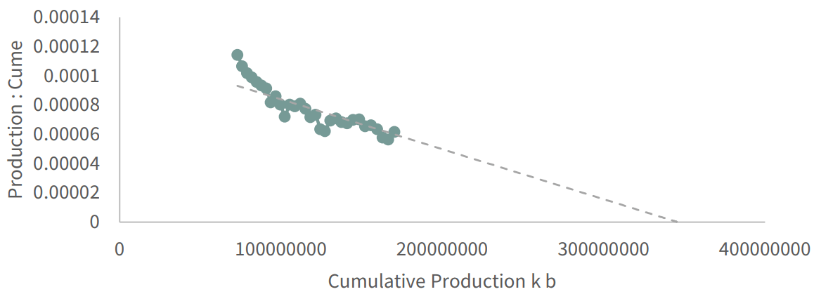
We next computed an expected production profile for Saudi Arabia based on the Linearization. This profile suggests that between 2018 and 2077, Saudi Arabia will produce 158 bn bbl – very much in line with the DeGolyer & MacNaughton audited figure. By 2077, the model predicts production will have fallen from 9 mm b/d today to only 3.1 mm b/d, with declines of 4% per annum. Aramco claims that post-2077, Saudi reserves will still total 53 bn bbl. However, we believe this is mathematically impossible. If 2077 production stands at 3.1 m b/d, and it declines by 4% per year, as suggested by our Hubert Linearization, then cumulative production from 2077 forward would never exceed 28 bn bbl.

Assuming the “too small, too remote” fields do not exist, and total reserves post-2077 total 28 bn and not 53 bn bbl (as reported in the summary), then Saudi’s ultimate recoverable reserves are 340 bn bbl, of which 52 % have been produced as of 2024. The Saudis are now past their halfway point in producing their recoverable reserves. Under this scenario, production cannot grow from here, and outright declines should be expected at any time.

Although a flurry of interest surrounded Mr. Simmons’s book nearly twenty years ago, few energy analysts pay attention to the Kingdom’s geological issues today.

FIGURE 2 Saudi Production Profile

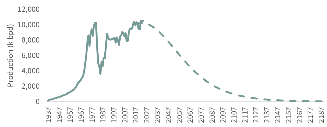
Although most analysts incorrectly interpreted the Saudi news as proof of “peak demand,” we take a different view: Matt Simmons was not wrong, merely early. We believe the recent announcement to abandon its growth targets is the first sign our analysis was correct, as outlined in 2019 in three essays-3rd Q 2018, 1st Q 2019, and 2nd Q 2019–, and that sustained Saudi Aramco production declines are much closer than anyone anticipates.

Is US Oil Production Surging?

The biggest mystery in oil markets surrounds the apparent surge in US production. At the beginning of 2023, we predicted shale growth would slow dramatically. Since 2010, shale oil production has grown by an astounding 8.3 m b/d. Including natural gas liquids, shales added 13 m b/d, representing nearly all non-OPEC growth. The Permian was the main growth driver in recent years, adding 5 m b/d of crude alone. The US shales met more than 100% of global demand growth since 2010.

We argued that while the shales were likely the most prolific source of crude in history, immense was not the same as infinite. We developed sophisticated neural network models to help us understand the ultimate recovery of the various basins and predict when the shales would plateau and eventually roll over. We concluded the immense pick-up in drilling productivity between 2016 and 2018 did not come from improved drilling techniques, as widely advertised, but rather from focusing on the most productive areas of the fields. Instead of turning mediocre acreage into highly profitable wells, the industry was aggressively drilling out the best parts of their resource – a process known in the mining industry as “high-grading.” Such practices cannot go on forever, and we correctly predicted the Eagle Ford and Bakken would begin showing signs of strain in 2019, while the Permian would likely plateau and eventually roll over sometime in either 2024 or 2025. By the start of 2023, our models suggested the Permian would probably see its growth slow dramatically within twelve months and may begin declining as early as the start of 2024.

Without the shales, it seemed impossible that US production would continue to grow. From January to December 2022, US crude production rose by a robust 700,000 b/d. We predicted this growth slow dramatically as 2023 progressed. Instead, according to the Energy Information Agency (EIA), US growth accelerated. By November 2023, the last for which wehave available data, the EIA claims US crude production was up 930,000 b/d year-on-year, while natural gas liquids added another 600,000 b/d. Taking their cues from the EIA, the International Energy Agency raised its estimates for 2023 US liquids production (including NGLs) by 400,000 b/d, implying year-on-year growth of 1.5 m b/d. According to the figures, 2023 represented the fourth most robust year for liquid growth in US history.

However, as we studied the data more closely, we have strong reason to believe it is simply incorrect. Instead of accelerating growth, our analysis suggests US liquids growth is overstated by nearly 30% while crude growth is overstated by 40%. Most importantly, our analysis tells us growth slowed dramatically throughout 2023 and is at risk of turning negative on both a year-on-year and sequential basis as early as March or April. If we are correct, the implications will be tremendous. Instead of surging, the only material source of non-OPEC production growth is grinding to a halt. Incredibly, we have seen very few analysts comment on the discrepancy, leading us to believe investors are poorly prepared or positioned.

The discrepancy centers around a restatement of government data in the summer of 2023. In March last year, newly appointed EIA Administrator Joesph DeCarolis took to Twitter to discuss the agency’s growing “adjustment factor.” The EIA reports the sources, uses, and inventory changes for crude and petroleum products in the monthly data. While stockpiles are measured directly, production, demand, and net imports are estimated. As a result, each month, the EIA must include an “adjustment factor” that reconciles supply and demand with changes in inventory levels. Between 1981 and 2016, the adjustment factor averaged 140,000 b/d; however, by February 2023, the figure had exploded to 840,000 b/d. Mr. DeCarolis outlined his intention to improve the reporting and “explain” the massive balancing item, which had grown to represent nearly 6% of US crude production.

FIGURE 3 EIA Crude Adjustment Factor

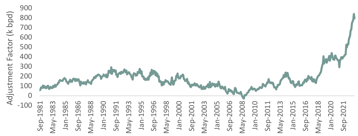
In his tweet, Mr. DeCarolis identified two key culprits. First, field production was being chronically under-reported. Second, operators were capturing and blending a refinery by-product, essentially creating a new unmeasured stream of crude-like liquids that could be fed back into the downstream process.

In July 2023, the EIA began explicitly breaking apart crude blending (“crude transfers”). As a result, the remaining adjustment factor fell by half and began reflecting only the under-reporting of field-level production. On the surface, this may sound bearish. For every month starting in at least January 2022 (the start date of the published revisions), the EIA was likelyunder-reporting production by 350,000 b/d on average.

However, upon closer inspection, adding the under-reported crude back to field production changed the growth trajectory entirely. Instead of pumping 11.9 mm b/d in 2022, the US likely produced 12.3 m b/d of oil. In 2023, instead of pumping 12.9 m b/d, the US probably made 12.8 m b/d. In other words, instead of growing by 1 m b/d last year, US crude production growth likely slowed to only 600,000 b/d.

Focusing on the monthly figures paints an even more dire picture. According to the headline figures, year-on-year US crude growth started and ended the year at a healthy 1 m b/d. However, adding back under-reported field production suggests US crude growth started 2023 at 1.4 m b/d and slowed to a mere 311,000 b/d year-on-year by December 2023. In August 2023, the headline figure showed a year-on-year increase of 1.1 m b/d, while the adjusted figure showed a year-on-year decline – the first since COVID-19.

Instead of showing steady and robust growth, our analysis suggests year-on-year US crude production growth will be slowed by 78% throughout 2023 – just as we had predicted last year.

These results are consistent with the other data we study. The total reported shale crude production started in 2023, growing at a healthy 700,000 b/d year-on-year. By December 2023, growth had slowed by 30% to less than 500,000 b/d. Furthermore, most shale growth came from a one-time liquidation of drilled but uncompleted wells in the Bakken. In the Permian – the main growth driver in recent years – crude production growth went from 635,000 b/d year-on-year in January to 100,000 b/d by December – a deceleration of nearly 85%. The US oil-directed rig count fell by 20% throughout 2023, making it highly unlikely US growth could have remained as robust as the headline figures suggest. Most importantly, the slowdown is consistent with our neural network, which tells us that over half of all recoverable reserves have been produced in every major shale basin.

If our analysis is correct, total US crude production may begin to decline sequentially as soon as the second quarter. By the end of 2023, production may be lower by nearly 1 m b/d. US crude production could fall by 470,000 b/d for the entire year compared to 2023. Although NGLs will likely grow, we do not expect it will be enough to offset crude declines. Total US liquids production (including NGLs) could average 19.3 m b/d this year, unchanged from 2023.

FIGURE 4 Headline US Crude Production Estimate

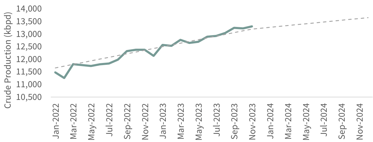
Investors have not incorporated the slowdown in their estimates. The IEA expects total US liquids to grow by 800,000 b/d this year – representing the world’s largest single source of growth. If we are correct, other markets will be much tighter than anyone expects within several months.

FIGURE 5 Adjusted US Crude Production Estimate

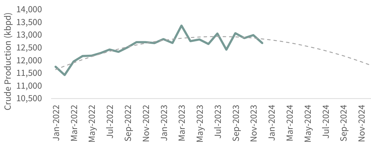
Over the last twelve months, oil markets have been broadly balanced. OECD commercial inventories drew a modest 100,000 b/d throughout the year. Looking forward, the IEA expects a surplus of nearly 800,000 b/d; however, we disagree. First, we believe the IEA is again underestimating demand, as evidenced by the return of the “missing barrels.” As our readers know, “missing barrels” occur when, according to the IEA, liquids that are neither consumed nor added to inventory are produced. Over the past twenty years, “missing barrels” have often predicted future upward revisions to demand. Last year, the IEA’s missing barrels averaged 400,000 b/d. In the fourth quarter, they reached a very large 700,000 b/d. We believe the IEA is underreporting demand again, especially as we enter 2024. Even if the US shales moderate from 4Q23 levels to an average of 500,000 b/d, the IEA’s expected surplus will fall to only 300,000 b/d.

Moreover, as discussed, the IEA expects US liquids production to grow by 800,000 b/d, whereas our analysis suggests production may be flat in 2024 compared with 2023. If we are even halfway right, oil markets will be in deficit for the fourth consecutive year. Both commercial and government inventories remain below average, leaving markets vulnerable to an unexpected move higher. Speculators hold nearly the lowest level of net-length in twenty years.

We previously predicted privately that if oil markets became tight, governments would release vast quantities from their strategic petroleum reserves to keep prices low. Although we never wrote about our predictions, they were proven correct in 2022 and the first half of 2023. Given the upcoming election, we would not be surprised if the Administration considered releasing further barrels from the SPR – something we would consider a massive mistake. Although this action might depress prices in the near term, we would use further SPR releases to prove the oil market is tighter than expected and exploit the weakness as a buying opportunity.

The only source of non-OPEC growth is grinding to a halt; we believe demand will again surprise the upside in 2024, and inventories, artificially boosted by SPR releases over the last two years, will begin to draw again strongly. Investors will be forced to take notice.

Is Gas the New Uranium?

Five years ago, we became uranium bulls. We explained how the market had quietly slipped into a structural deficit, with reactor demand outstripping mine supply. Fuel buyers used so-called “secondary supplies” to fill the gap -notably large commercial stockpiles accumulated following the 2011 Fukishima nuclear accident. At the time, investors did not pay uranium any attention at all. The premiere Western uranium producer, Cameco (CCJ), changed hands at $9 per share – 20% below its tangible book value – and held nearly $800 mm of cash on its balance sheet. By the first quarter of 2019, no uranium company on any exchange sported a double-digit stock price – a sign that investors had given up on the industry. Investor attitude is entirely different today. Bloomberg consistently reports on structural deficits. Instead of trading for $9, a share of Cameco now changes hands for more than $50.

Why start our natural gas essay with a discussion of uranium? We believe today’s North American natural gas market resembles that uranium market : despite widespread investor pessimism, it too is about to slip into “structural deficit”. Careful research and a differentiated outlook may reward the enterprising natural gas investor just as large profits accrued to the uranium investor back in 2018.

North American natural gas collapsed after peaking at nearly $10 per mmbtu in August 2022. Many analysts point to surging supply; however, this fails to capture the whole story. In June 2022, the Freeport LNG export terminal on Quintana Island, Texas, caught fire, halting operations. The terminal did not resume full output until March 2023. Freeport exported two bcf/d, representing nearly 2% of total US demand. We estimate the fire affected about 600 bcf of export demand over the 100 days the terminal remained closed. As a result, US natural gas inventories grew by 700 bcf compared with long-term seasonal averages between June 2022 and March 2023 – 85% of which was attributable to the Freeport fire. Making matters worse, the 2022/2023 North American winter was the fourth mildest since records began 130 years ago.

Once Freeport resumed operations, natural gas inventories began to draw sharply. By the end of the injection season on November 1st, 2023, nearly 90% of the excess inventory had been worked off. Unfortunately, the start of the 2023/2024 withdrawal season has been mild again. Since November 1st, North American temperatures have consistently registered 10% warmer-than-normal, reducing heating demand and swelling inventories relative to normal.

North American storage sits nearly 250 bcf above seasonal averages, driving prices back to $2.23 per mmbtu – nearly 80% below its energy equivalent compared with oil and seaborne gas.

Although weather explains most of the recent inventory glut, many analysts blame growing production, which we believe to be incorrect. For the past decade, three fields have been responsible for nearly all US natural gas supply growth: the Marcellus, Permian, and Haynesville. These three basins represent almost 60% of total US gas production. After such prolific growth, most analysts seem to believe these fields will grow forever. We disagree. Instead, our models suggest US production will experience unanticipated declines over the next several years.

We believe enough data exists to attempt to model future US shale gas production, and the conclusions are dire. Using our proprietary neural network, we have estimated the major shale basins’ Tier 1 drilling inventory and expected ultimate basin recovery. Like a sizeable conventional field, we believe that a shale basin’s production will peak when half its recoverable reserves have been produced. Furthermore, we can monitor ongoing drilling productivity in real time to help confirm we are traveling down the right path.

Our models conclude that the Marcellus, Haynesville, and Permian are plateauing and each could experience declines within the following year. By 2026, we expect these fields will resemble two of the earliest shale fields – the Barnett and Fayetteville.

FIGURE 6 Barnett and Fayetteville Production

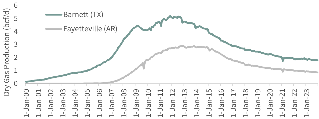
Our neural network helped us identify two indicators hinting at forthcoming production declines. First, we can estimate when producers will have produced half by estimating a field’s ultimate recoverable reserves. Historically, this has correlated very well with a basin’s maximum production rate. Next, we evaluate how many of a basin’s most prolific wells (so-called Tier 1) producers have drilled. Based upon historical precedents in the Barnett, Fayetteville, Eagle Ford, and Bakken, we observe that production begins to decline once operators have drilled 60% of the best wells.

We find it helpful to monitor a real-time indicator of basin health. If a field is about to decline, we should expect its average well productivity to fall, suggesting its top Tier 1 wells inventory has been mostly exhausted. Observing two consecutive years of sustained productivity declines increases our confidence that our estimate of Tier 1 inventory was correct.

How did our framework do with the Fayetteville and Barnett – the first two shale gas basins to peak and roll over? In the case of the Fayetteville, our neural network suggests the basin will ultimately recover ten tcf. A Hubbert Linearization, an older reserve estimation technique, arrives at a similar figure. Just as our theories would predict, the Fayetteville peaked at 3.0 bcf/d once half of the ultimate recoverable reserves were produced. Production started declining sharply once 60% of our estimated Tier 1 wells were drilled. In the Barnett, our neural network estimated total recoverable reserves of 23 tcf-a figure again confirmed using a “Hubbert Linearization.” Just like the Fayetteville, production peaked in 2012 at 5.0 bcf/d, once half the reserves had been produced, and 60% of the best wells had been drilled. The Fayetteville and Barnett helped us properly calibrate our understanding of shale basins and inform our views of the Marcellus, Permian, and Haynesville.

Our neural network predicts that the Marcellus and Haynesville will ultimately recover 130 and 75 tcf, respectively. A Hubbert Linearization of the Marcellus confirms this estimate. Unfortunately, a similar analysis of the Haynesville is more challenging. Haynesville production peaked in 2012 at 7.5 bcf/d, declined over the next three years due to low prices, and staged a second material ramp-up. The Haynesville’s irregular profile makes a traditional Hubbert Linearization difficult; however, our neural network works off actual well data and is immune from such disruptions.

By mid-2022, the Marcellus had produced 68 tcf – slightly more than half its ultimate recoverable reserves. From 2012 to 2022, Marcellus dry gas production grew on average by 2.1 bcf/d per year. Since mid-2022, annual growth has only averaged 0.1 bcf/d – a 95% slowdown. By late 2023, the Haynesville had produced 38 tcf, equivalent to half of its recoverable reserves. From 2018, when it began its second production surge, until August 2023, Haynesville growth has averaged 1.8 bcf/d per year. Since August, growth has slowed by 77% to only 340 mmcf/d annualized. Our framework suggests field depletion in both major basins is responsible for the slowdown. We do not believe the Haynesville will be able to start growing again, unlike what happened back in 2017. When the Haynesville first peaked in 2012, it had produced less than 10% of its recoverable reserves. If we had our models back then, we would have known the field could stage a massive recovery. No such luck this time. Instead, we believe the Marcellus will turn from plateau to outright decline within a few months. In the Haynesville, we expect 2024 production will only grow modestly before declining sequentially later this year.

The remaining Tier 1 inventory serves to confirm our prediction. The Barnett and Fayetteville moved from plateau to decline once operators drilled 60% of their best wells. Presently, operators in both the Marcellus and Haynesville have also drilled 60% of their best locations. As a result, we expect the Marcellus will soon begin to decline. Moreover, the Haynesville may move more quickly from slowing growth to plateau and ultimately decline sooner than we expect.

Real-time well productivity data further confirms our outlook. In the Barnett and Fayetteville, drilling productivity peaked and declined twenty-fours months before the field reached maximum output, respectively. Productivity in both the Marcellus and Haynesville peaked in 2021 and has since slowed by between 15 and 20%. Production declines are imminent if the Marcellus and Haynesville follow the Barnett and Fayetteville.

Growth in associated gas production from the Permian is slowing rapidly as well. For those interested, please refer to our 1Q23 essay: “The Permian Is Depleting Faster Than We Thought.” We will also release a video analysis of the Permian in the coming months.

Analysts remained fixated on the continued year-on-year growth in US gas production; however, few have commented on how quickly the growth has slowed. On a year-on-year basis, US dry gas production decelerated from six bcf/d to slightly over two bcf/d. Regarding demand, LNG export capacity will increase by six bcf per day over the next twelve months. All of this new demand is fully permitted and currently under construction. None is subject to the Biden administration’s recent proposed moratorium on new LNG terminals, which only applies to future planned projects. Our modeling suggests dry gas production will not be able to meet the new demand. As a result, we expect the US natural gas market will slip from surplus to deficit sometime later this year. With international gas trading for $12 per mmbtu (four times the domestic price), traders will aggressively bid US prices higher to take advantage of the arbitrage.

As always, the weather remains a wild card. However, even if the remainder of the North American winter is mild, we believe the market will become tighter within twelve months. Any weather-related weakness presents an excellent buying opportunity. North American gas today resembles uranium in 2018: the market is about to shift from surplus to deficit, yet investors remain bearish.

Uranium Mine Supply Faces Challenges

On January 12th, Kazatomprom (OTC:NATKY), the publicly traded Kazakh national uranium company, shocked the markets by announcing it could not meet its production guidance for 2024 and 2025. That announcement represented a dramatic about-face after years of stated planned capacity expansions. In August 2022, Kazatomprom increased its expected 2024 production by four to six million pounds in response to significant strength in their forward sales book. Following the announcement, Kazatomprom expected to produce between 55 and 56 mm pounds in 2024 – an increase of 11 mm pounds over 2023’s estimated output. The company followed this up with a second announcement on September 29th, 2023, again increasing production guidance for 2025:

“Consistent with our market-centric strategy, our intentions to return to a 100% level of Subsoil Use Contracts production volume in 2025 is primarily driven by our strong contract book and already growing sales portfolio against a conservative 2023-2024 production scenario. As we are seeing a clear sign that the industry has entered into the new long-term contracting cycles, driven by the recognition of the restocking needs, Kazatomprom, with its best-class and lowest-cost mines, is absolutely prepared to respond to these improving marketing conditions. Our current contact book provides sufficient confidence that the additional volume in 2025 will have a secure place in the market and be needed to fulfill future contractual obligations.”

Kazatomprom announced they would boost 2025 production to between 67 and 69 mm pounds to meet strong demand – a significant 15 mm pound increase above the expected 2024 output. Our 4Q23 letter expressed skepticism over Kazatomprom’s planned expansion, citing a potential sulfuric acid shortage.

Our concerns were justified. In their January 19th announcement, Kazatomprom warned that a lack of sulfuric acid and ongoing construction delays have made their 2024 and 2025 production guidance impossible. On February 1st, Kazatomprom officially lowered their 2024 production guidance by nearly 20%, from 56 to only 46 to 50 mm pounds- a decrease of almost 10 mm from previous guidance. Although the company did not discuss 2025 production, we believe their 67 to 68 mm pound target will be impossible.

Uranium rallied sharply to $90 per pound during the fourth quarter, driven by solid utility buying. Even after the recent activity, global utilities remain woefully under-contracted compared with historical norms. In past letters, we warned that utilities would need to re-enter the market to meet their needs – it appears that time has now arrived. Following Kazatomprom’s surprise announcement, uranium surged another $16, hitting a cycle-high of $106 per pound.

Although the uranium market is notoriously opaque, we believe Kazatomprom already sold forward some portion of its previously expected 25 mm pounds of 2024 growth. Depending on how much uranium Kazatomprom has already committed, it may have to buy material in the spot market to fulfill its contract obligations.

The world’s two largest producers are now both short of uranium. On September 3rd, Cameco, the world’s second largest uranium producer, announced expected production shortfalls at McArthur River and Cigar Lake, totaling 3 mm pounds. Given that before their recent announcements, Cameco and Kazatomprom were likely fully contracted for the next four years, we believe both companies have committed to selling more uranium than they can produce. If correct, both companies may have to buy material on the spot market, driving higher prices.

Our 2Q23 letter explained how uranium had entered uncharted territory. Since the end of World War II, there existed, without exception, a material inventory cushion of secondary supply to bridge any period where reactor demand outstripped mine supply. Based upon our modeling, and the fact that financial buyers have emerged to compete with utility buyers for scarce spot volumes, we concluded these inventories would soon deplete entirely, making this cycle different from past bull markets.

Uranium has now slipped into a structural deficit and is about to get even tighter. Demand continues to grow, while production is beginning to disappoint.

Although we believe new production will eventually end the bull market, we expect very little new mine supply for the next several years. In previous letters, we predicted the uranium bull market would soon become chaotic- that period is now upon us.

New Copper Technologies

Copper demand was extremely strong in 2023, growing 7.3% year-on-year over the first ten months, according to the World Bureau of Metal Statistics (WBMS). Nearly all copper demand growth came from the non-OECD world. As in recent years, China led the group higher. Although many remain concerned about perceived weak Chinese economic output and ongoing problems in their property sector, Dr. Copper is undeterred.

Countless analysts have warned for years that China is over-consuming copper, but we disagree. These analysts often model annual copper demand as a function of real GDP, which we believe is a mistake. Unlike oil, which economies consume, copper is “installed.” Like any capital good, “installed copper” will last decades. Instead of looking at annual copper consumption (a flow, for those accountants among you), we prefer to analyze an economy’s total installed copper base, net of a depreciation allowance (a stock). By studying the relationship between its cumulative installed copper base and real GDP, we concluded that China is exactly where it should be for an economy of its size. Sporting a real per capita GDP of $12,500, China has approximately 260 pounds of installed copper for every man, woman, and child. As you can see from the chart below, China’s installed copper base is very much in line with other countries at similar levels of economic development.

FIGURE 7 Installed Copper S-Curve

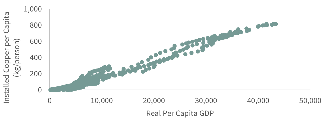
Chinese officials have repeatedly expressed a desire to avoid the dreaded “middle-income” trap. For China to succeed in becoming a wealthy country, it must grow its real GDP to between $18 and $20,000 per capita. To reach this target, they must increase their installed copper base from 260 pounds per person currently to 360 pounds. With a population of 1.4 bn, China will need to install an additional 100 mm tonnes of copper to reach its economic goals. Assuming China grows at 5% per year, it will reach $19,000 per capita GDP by 2035. Annual copper consumption will need to average 15 mm tonnes per year for the next ten years in order to reach these targets.

Moreover, as dramatic as these projections are, they represent only the minimum level of copper investment required to meet their targeted level of GDP based on historical precedents. If China continues its large-scale renewable energy build-out, which is hugely copper-intensive, our projections may well prove conservative.

India, too, has reached an inflection point in its copper demand. Historically, Indian copper demand growth was relatively modest. With much lower levels of per capita GDP, India did not yet require an extensive copper base installation. That has now changed. Before 2020, India’s real GDP remained stubbornly below $2,000 per person. Over the last three years, economic growth accelerated, and we now estimate real GDP will reach $2,800 per capita by the end of the year. As our models predicted, Indian copper demand has started to surge.

FIGURE 8 Indian Copper Consumption

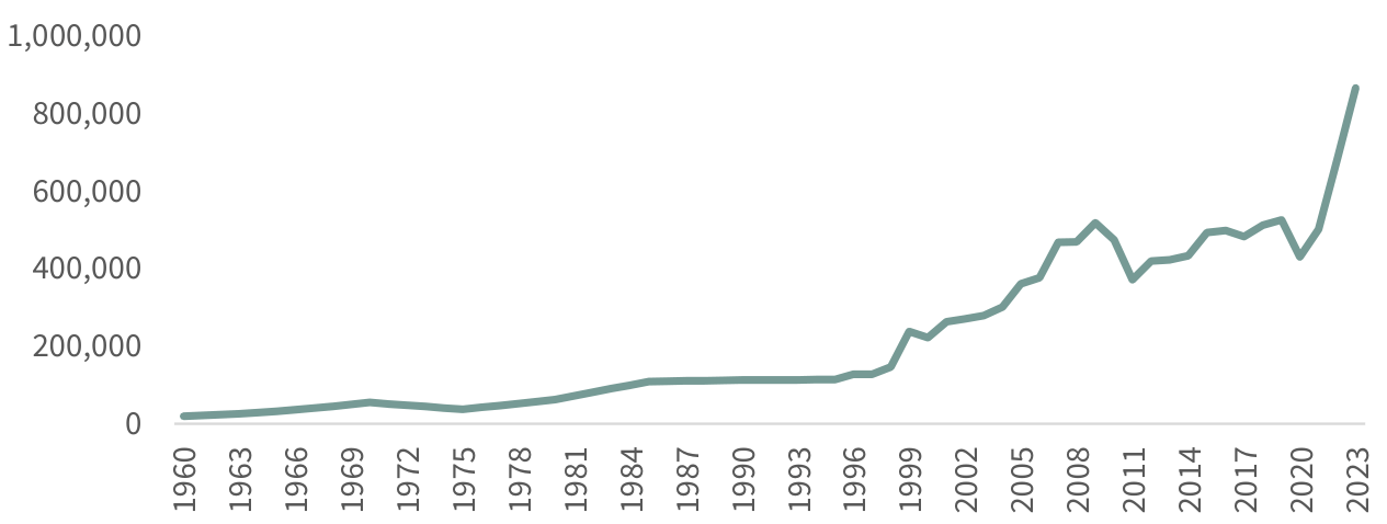
Indian copper consumption nearly doubled in the last two years alone. Despite the strong growth, India’s installed copper base remains woefully meager. By comparison, China had 45 pounds of copper installed per person when it reached $3,000 of real per capita GDP in 2003. Presently, we estimate India’s per capita copper base is only 15 pounds. Indian economic growth is expected to remain around 6% for the foreseeable future, which, along with its very low starting installed copper base, should increase its annual copper consumption nearly four-fold from current levels over the coming decade. Although this sounds extreme, Chinese copper demand increased by over four-fold between 2000 and 2010. Few analysts have commented on surging Indian copper demand; we believe this will soon change. Our models tell us India has finally emerged as a significant player in the copper market as we progress through the decade.

Another large non-OECD country has caught our attention: Indonesia. On September 20th, 2022, an article appeared in the Financial Times: “Indonesia’s Expected Success Story.” After years of disappointment, the authors argued that Indonesia boasted a booming economy and stable government. The economy had grown by 5% for two consecutive years and managed through COVID-19 and Russia’s invasion of Ukraine with only mild inflation. The rupiah was among the best-performing Asian currencies and the stock market was hitting all-time highs. A second article appeared in the Financial Times more than a year later: “Is Indonesia Finally Set to Become an Economic Superpower?” Significant infrastructure investment combined with a commodity export boom resulted in another year of growth that surpassed expectations. Leading economists projected that Indonesia could become the world’s seventh-largest economy by 2030.

Consistent with these articles (and of particular importance to us), Indonesian copper demand is now surging. For many years, Indonesia has been caught in a classic middle-income trap. After reaching a per capita GDP of $2,000 in 2005, it took the country nearly another twenty years to exceed $4,000. Indonesian prosperity was hampered by political instability, widespread corruption, and notable investment shortfalls – all of which have been covered in the press. However, we believe another factor contributed to the country’s lackluster growth: a shortage of installed copper, a dark irony given that Indonesia is home to Grasberg and Batu Hijau – two of the largest copper mines in the world. Nevertheless, when Indonesia first reached $2,000 of real per capita GDP in 2005, we calculated their total installed copper base only totaled 13 pounds per person – far too low for sustained economic growth. By comparison, China had 30 pounds invested per person in 2000 when it reached $2,000 of real per capita GDP.

Since 2005, Indonesia’s installed copper base has doubled to 35 pounds per person, still far too low. Anyone who has experienced Jakarta’s gridlock will agree that Indonesia’s investment in infrastructure remains terribly inadequate, a problem President Joko Widodo has prioritized. Massive new projects are underway, including the controversial plan to move the national capital from Jakarta to Kalimantan. Our models suggest Indonesia requires at least 80 pounds of installed copper per person to sustain a per capita real GDP above $4,000 – some 160% above present levels.

Indonesia faces another period of political uncertainty in the near term as President Widodo steps down later this year. However, we believe the current strong trends in copper consumption will persist, regardless of the country’s leadership. Although uncertainties remain, Indonesia requires much more installed copper to escape the middle-income trap. Based on current trends, Indonesia is quickly reaching its inflection point in copper consumption, similar to China in 2003 and India presently. If Indonesia ever earned $10,000 of per capita real GDP, we estimate it would have to increase its installed copper base from 35 to 200 pounds per person. Given its population of 275 mm, even if it takes another 15 years, assuming 5% economic growth, we expect Indonesia will consume over 1 mm tonnes annually – five times the current rate. In future letters, we will closely monitor Indonesia’s copper consumption, but it represents yet another potential source of incremental demand, which most analysts completely ignore.

In the short term, we remain incredibly bullish. Strong demand, supply disappointments, and meager exchange inventories leave the market susceptible to price spikes. Over the longer term, however, we are more cautious. Analysts have become universally bullish over a lack of long-term copper mine supply growth. In our last letter, we discussed Robert Friedland and the potentially disruptive technologies he will unleash on the hard-rock mining industry.

Mineral exploration has remained remarkably unchanged over the last 150 years. Geologists still often walk diligently, looking for the rock and soil alterations that suggest a deposit may be near the surface. Although induced-polarization geophysical studies have helped somewhat, their practical resolution only extends a few hundred meters deep. For the most part, geologists remain unable to see anything deeper. Any deeper discovery has primarily occurred accidentally, chasing a surface anomaly to depth. The mining industry has failed to replicate the advanced exploration tools perfected by the oil and gas industry over the last fifty years, until now.

With the introduction of Ivanhoe Electric’s Typhoon survey, hard-rock geologists can, for the first time, image mineral deposits several thousand meters below the surface. Unsurprisingly, 80% of all copper mine supply comes from deposits discovered within 200 meters of the surface – that is how deep the geologists could “see.” With Typhoon, that has changed. We know that copper porphyries exist at depths greater than 200 m, as several have been discovered by accident. However, the industry has never been able to explore for these large ore bodies efficiently from the surface.

Mr. Friedland is not the only one bringing “disruptive” exploration technologies to bear. Privately held KoBold Mining has had some initial success using artificial intelligence to help identify economic mineral deposits. On February 5th, the company announced a self-proclaimed “huge” copper discovery at its Mingomba project in Zambia. Although details remain scarce, CEO Josh Goldman has compared his discovery with Friedland’s Kakula, across the border in the Democratic Republic of Congo – arguably the most important copper discovery of the past two decades.

New technologies are not just limited to exploration. Using the same “pulsed power” technology that enables Typhoon, Mr. Friedland has also advanced a new technology that could disrupt how companies drill through, mine for, and crush rock. “I-Rox” uses pulsed power to pull rock apart from the inside, instead of being crushed from the outside-resulting in huge energy savings and cost. The implications could be transformative. There exists today huge quantities of low-grade sulfide ores-ores that are presently uneconomic to mine and process because of their low grades.

If I-ROX can deliver on its promise to reduce energy consumption by an order of magnitude, mining companies could quickly begin developing previously unprofitable projects. Given the vast amount of identified but uneconomic copper deposits, I-ROX could single-handedly change the supply dynamics of the industry. The copper industry has an interesting recent historical parallel: the introduction of solvent-extraction / electro-winnowing (SX/ EW) in the late 1980s. Before introducing SX/EW, copper miners could not economically unlock their vast inventory of low-grade oxide deposits. Once the industry adopted SX/ EW, oxide copper surged to nearly 20% of total mine production in just ten short years, resulting in a huge price-depressing glut.

Mr. Friedland and I spoke at a mining conference in New York City in late January. In his remarks, he used the term “disruptive” at least six times when describing Typhoon and I-ROX. We could not agree more.

As if Mr. Friedland has not been busy enough, Ivanhoe Mines, the operator of Kamoa-Kakula in the DRC, recently announced a new world-class discovery adjacent to their existing operation with its “Western Forelands.” The company recently announced two discoveries: Kiala and Kitoko. In addition, Ivanhoe Mines released an initial resource estimate for the Mokoko deposit, first reported in 2018. With an initial resource of nearly 5 mm tonnes of indicated copper at an average grade of 3.5% using a 1% cut-off, Mokoko already ranks as one of the most significant and highest-grade copper discoveries of the past decade. The deposit remains open in nearly every direction and we expect it will grow as the company continues drilling. Given its high-grade core and volume, it is easy to see Makoko becoming a large 200,000 tonnes producer based on its initial resource alone.

Ivanhoe Mines also announced a small maiden resource for Kiala of 200,000 tonnes of contained copper grading 2.67% at a 1% cut-off. Although small, the deposit helps validate the geological model and will grow from here. Lastly, the company announced drill results from the high-grade Kitoko discovery. These results were fascinating, as we believe they open up a new potential geological trend and further confirm Ivanhoe’s understanding of the Western Forelands Basin. All these Western Foreland discoveries were made without any help from Mr. Friedland’s Typhoon technology.

Before the Kitoko discovery, exploration geologists believed copper mineralization was primarily hosted in a sandstone layer rising above the basement rock. Kitoko validates the theory that copper can be hosted directly adjacent to the conglomerate bedrock. As a result, an astonishing 175 km of additional strike length now has meaningful exploration potential. One particular drill hole at Kitoko returned a 5-meter intercept grading an astounding 11.6% copper, suggesting the deposit has at least the potential for an ultra-high grade zone similar to those found at Kakula, a mere 25 km away.

The potential in the Western Forelands is enormous. Ivanhoe Mine’s DRC copper production has already affected the global copper mine supply. For the first ten months of 2023, global mine supply grew by 400,000 tonnes, nearly half attributable to the Kamoa-Kakula’s Stage 2 expansion. Stage 3 will come online by the end of 2024 and will add another 200,000 tonnes of copper mine supply.

Although the Western Forelands will not come online for several years, we must monitor the project closely. Most analysts are convinced that copper mine supply can never grow, but we believe we may be on the verge of a significant investment boom, led by a whole new exploration cycle-led primarily by new technologies.

Grain Traders Approach Record Bearish Levels

Over the last sixteen months, weak grain prices have left traders extremely bearish, especially in markets unaffected by the ongoing El Nino. Due to El Nino, India, southern Asia, and West Africa have suffered near drought conditions since June 2023. As a result, the main crops in these regions, notably cocoa and palm oil and, to a lesser extent, wheat, have seen prices fall by much less.

We study the positioning of both speculators and commercial traders on the various futures exchanges. Often, when commercial grain traders hold net long positions, grain prices rise. Commercial traders represent the “smart” money and, under normal market conditions, maintain a net short position to hedge their long physical inventory. A cereal maker must hold large corn inventories and will turn to the futures market to hedge this exposure, resulting in a net short commercial position. On rare occasions, commercial traders will close out their hedges and maintain net long positions. Although rare, a net long commercial position suggests that the “smart” money is worried about future crop supply and is a bullish indicator. Since a net short position must offset every net long position, speculators (i.e., trend followers) are usually net long when the commercials are net short. When the commercial traders turn net long, the speculators will often turn net short, taking the other side of the trade.

FIGURE 9.3 Corn Commitment of Traders

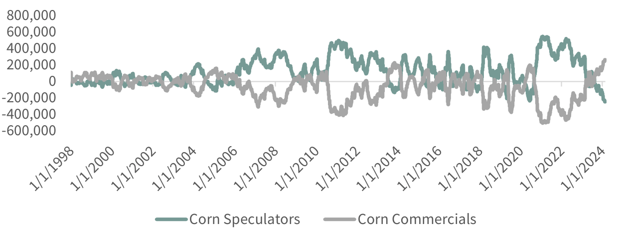
Having commercials net long and speculators net short has in the past indicated a significant buying opportunity. Speculators in corn and soybeans now have near-record net short positions, rivaling the extremes last seen in 2019 and 2020 for soy and corn, respectively. Wheat speculators are also short, albeit not at quite the same extreme levels as corn and soy. Corn and soy commercial traders are at near-record net long positions. Wheat commercial traders are also significantly net long, but not at the same extreme levels as corn and soy.

The last time corn speculators were this net short and commercials were this net long was June 2020, at which point corn bottomed at $3.15 per bushel. Corn was 160% higher two years later, reaching $8.15 per bushel. The last time soy speculators were this net short was May 2019, at which point prices bottomed at $8.00 per bushel. Over the next two years, soy more than doubled. In wheat, speculators were this net short last in January 2018, at which point prices bottomed at $4.00 per bushel before surging nearly four times over the next four years.

FIGURE 9.2 Soy Commitment of Traderst

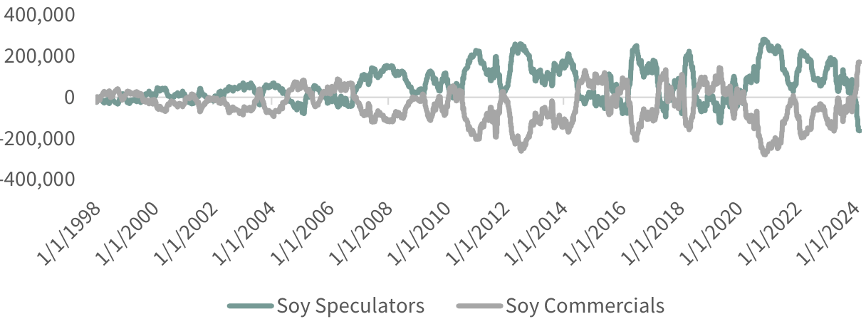
FIGURE 9.1 Wheat Commitment of Traders

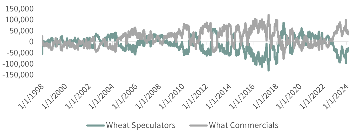
We believe the current positioning indicates that grain prices are poised to enter a potentially massive bull market. The eighteen-month sell-off is likely nearing an end. Investors should position themselves accordingly.

---

Registration with the SEC should not be construed as an endorsement or an indicator of investment skill, acumen or experience. Investments in securities are not insured, protected or guaranteed and may result in loss of income and/or principal. Historical performance is not indicative of any specific investment or future results. Investment process, strategies, philosophies, portfolio composition and allocations, security selection criteria and other parameters are current as of the date indicated and are subject to change without prior notice. This communication is distributed for informational purposes, and it is not to be construed as an offer, solicitation, recommendation, or endorsement of any particular security, products, or services. Nothing in this communication is intended to be or should be construed as individualized investment advice. All content is of a general nature and solely for educational, informational and illustrative purposes. This communication may include opinions and forward-looking statements. All statements other than statements of historical fact are opinions and/or forward-looking statements (including words such as “believe,” “estimate,” “anticipate,” “may,” “will,” “should,” and “expect”). Although we believe that the beliefs and expectations reflected in such forward-looking statements are reasonable, we can give no assurance that such beliefs and expectations will prove to be correct. Various factors could cause actual results or performance to differ materially from those discussed in such forward-looking statements. All expressions of opinion are subject to change. You are cautioned not to place undue reliance on these forward-looking statements. Any dated information is published as of its date only. Dated and forward-looking statements speak only as of the date on which they are made. We undertake no obligation to update publicly or revise any dated or forward-looking statements. Any references to outside data, opinions or content are listed for informational purposes only and have not been independently verified for accuracy by the Adviser. Third-party views, opinions or forecasts do not necessarily reflect those of the Adviser or its employees. Unless stated otherwise, any mention of specific securities or investments is for illustrative purposes only. Adviser’s clients may or may not hold the securities discussed in their portfolios. Adviser makes no representations that any of the securities discussed have been or will be profitable. Past performance is not a guarantee of future results.

Click to enlarge

---

Original Post

Editor’s Note: The summary bullets for this article were chosen by Seeking Alpha editors.

Editor’s Note: This article discusses one or more securities that do not trade on a major U.S. exchange. Please be aware of the risks associated with these stocks.